To demonstrate tree classifiers we will start with the very simple example we used for GLM.
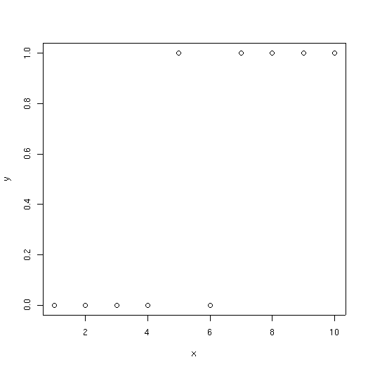
x <- 1:10
y <- c(0,0,0,0,1,0,1,1,1,1)
plot(x,y)
As you can see, at low values of x, species y is usually absent; at high values of x it is usually present. With a tree classifier, we try and find a series of splits that separates the presences from absences. In this example the dataset is artificially small; tree() usually will not produce splits smaller than 5 samples. So to make things work on this example we have to override some of the defaults as shown below.
To see the tree simply type its name.
test
node), split, n, deviance, yval, (yprob)
      * denotes terminal node

1) root 10 13.860 0 ( 0.5000 0.5000 )
  2) x < 4.5 4  0.000 0 ( 1.0000 0.0000 ) *
  3) x > 4.5 6  5.407 1 ( 0.1667 0.8333 ) *
The "root" node is equivalent to the null deviance model in GLM or GAM; if you made no splits, what would the deviance be? In this case we have 5 presences and 5 absences, so
-2 * 10 * log(0.5) = 13.86
The second branch has 4 samples, all absences, so the deviance associated with it is 0.
The tree keeps splitting "nodes" or branch points to make the resulting branches or leaves more "pure" (lower deviance).
There is a summary function associated with trees.
summary(test)
Classification tree:
tree(formula = factor(y) ~ x, control = tree.control(nobs = 10,
    mincut = 3))
Number of terminal nodes:  2
Residual mean deviance:  0.6758 = 5.407 / 8
Misclassification error rate: 0.1 = 1 / 10
The summary() function shows
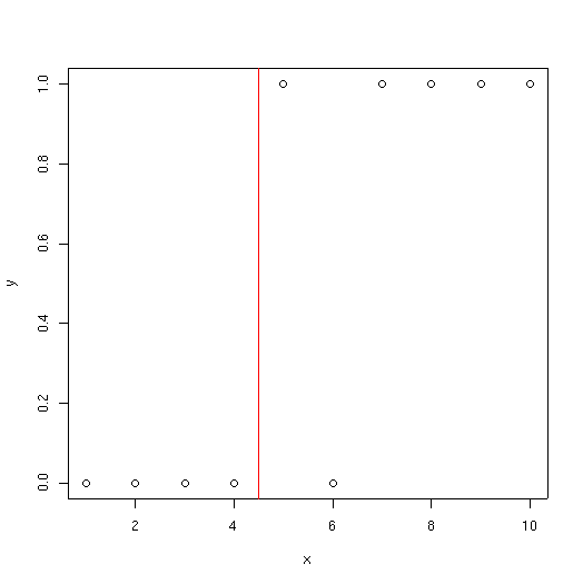
The following plot shows the split identified by the tree.
demo <- tree(factor(berrep>0)~elev+slope+av)
summary(demo)
Classification tree:
tree(formula = factor(berrep > 0) ~ elev + slope + av)
Number of terminal nodes:  15
Residual mean deviance:  0.4907 = 71.15 / 145
Misclassification error rate: 0.1125 = 18 / 160
demo
node), split, n, deviance, yval, (yprob)
      * denotes terminal node

 1) root 160 218.200 FALSE ( 0.57500 0.42500 )
   2) elev < 8020 97  80.070 FALSE ( 0.85567 0.14433 )
     4) slope < 20 89  62.550 FALSE ( 0.88764 0.11236 )
       8) slope < 2.5 35  39.900 FALSE ( 0.74286 0.25714 )
        16) av < 0.785 22  28.840 FALSE ( 0.63636 0.36364 )
          32) elev < 7660 11  15.160 TRUE ( 0.45455 0.54545 )
            64) elev < 7370 6   7.638 FALSE ( 0.66667 0.33333 ) *
            65) elev > 7370 5   5.004 TRUE ( 0.20000 0.80000 ) *
          33) elev > 7660 11  10.430 FALSE ( 0.81818 0.18182 )
            66) av < 0.455 6   0.000 FALSE ( 1.00000 0.00000 ) *
            67) av > 0.455 5   6.730 FALSE ( 0.60000 0.40000 ) *
        17) av > 0.785 13   7.051 FALSE ( 0.92308 0.07692 ) *
       9) slope > 2.5 54   9.959 FALSE ( 0.98148 0.01852 )
        18) av < 0.7 36   0.000 FALSE ( 1.00000 0.00000 ) *
        19) av > 0.7 18   7.724 FALSE ( 0.94444 0.05556 )
          38) elev < 7490 5   5.004 FALSE ( 0.80000 0.20000 ) *
          39) elev > 7490 13   0.000 FALSE ( 1.00000 0.00000 ) *
     5) slope > 20 8  11.090 FALSE ( 0.50000 0.50000 ) *
   3) elev > 8020 63  51.670 TRUE ( 0.14286 0.85714 )
     6) av < 0.055 7   9.561 TRUE ( 0.42857 0.57143 ) *
     7) av > 0.055 56  38.140 TRUE ( 0.10714 0.89286 )
      14) av < 0.835 36   9.139 TRUE ( 0.02778 0.97222 )
        28) av < 0.215 8   6.028 TRUE ( 0.12500 0.87500 ) *
        29) av > 0.215 28   0.000 TRUE ( 0.00000 1.00000 ) *
      15) av > 0.835 20  22.490 TRUE ( 0.25000 0.75000 )
        30) av < 0.965 12  16.300 TRUE ( 0.41667 0.58333 )
          60) slope < 2.5 6   7.638 FALSE ( 0.66667 0.33333 ) *
          61) slope > 2.5 6   5.407 TRUE ( 0.16667 0.83333 ) *
        31) av > 0.965 8   0.000 TRUE ( 0.00000 1.00000 ) *
Notice how the same variables are used multiple times, often repeatedly in a single branch
plot(demo)
text(demo)
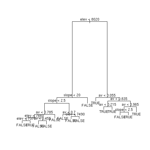
The height of the vertical lines in the plot is proportional to the reduction in deviance, so not all lines are equal, and you can see the important ones immediately.
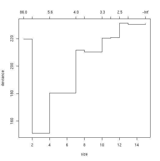
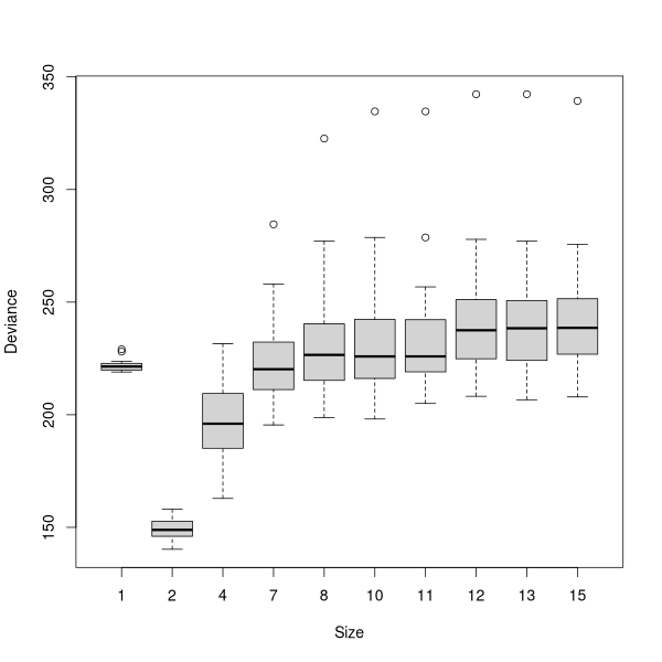
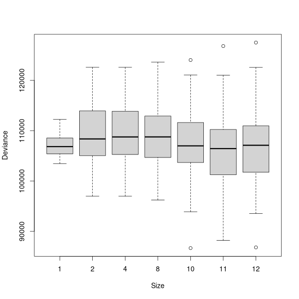
The curve (or jagged line) shows where the minimum deviance occurred with the cross-validated tree. Many people find these curves difficult to evaluate, as the stair-step curve seems ambiguous for a single value. For example, what is the value for X=4, ~150, or ~ 180? These curves are read as the last point along the line or any given X: thus at X=2, Y=147, not 220, and at X=4, Y=180, not 147.
In this case, the best tree would appear to be 2-3 terminal nodes. Actually, there was no test for 3 terminal nodes, only 2 and 4, so the straight line from 2 to 4 is a little misleading. So, we'll get the best tree with two terminal nodes.
The results of a cross-validation are stochastic, and every time you run the
cv.tree() function you will get somewhat different results. To
finesses this problem, the multi.cv() function (see below) can be used
to generate a boxplot of results.
In addition, note that the misclassification rate has gone up significantly.
The previous number was an optimistic over-fit number; this one is much more
realistic.
As you can see, the tree is remarkably simple with only two terminal nodes.
Surprisingly, it's fairly accurate. As you might remember from
Arguably, based on parsimony, we would want the smallest tree that has minimum
cross-validated deviance. As a special case, if the minimum deviance occurs
with a tree with 1 node, then none of your models are better than random,
although some might be no worse.
Alternatively, in an exploratory mode, we might want
the most highly-resolved tree that is among the trees with lowest deviance (as
long as that does not include the null tree with one node). For
the sake of example, lets go with a four node tree.
Notice that while the residual deviance decreased a little (0.722 vs 0.834),
the classification accuracy did not improve at all (23/160 misclassified).
Despite the apparent increase in detail of the tree, it's arguably actually no better.
Let's try an example with topographic position, this time using
Arctostaphylos patula.
For the sake of exploration I'm going to go with a slightly more complicated
tree than indicated bt cross-validation.
So, lets detach our bryceveg data frame, and attach the cover-class
midpoint data frame from Lab 1.
Exactly as we did for classification trees, we can cross-validate the regression
tree as well.
 To prune the tree, we use the prune.tree() function with a
best=n argument, where n = the number of terminal nodes we want.
demo.x <- prune.tree(demo,best=2)
This "pruned" tree is a tree object just like the others, and can be plotted or
summarized.
To prune the tree, we use the prune.tree() function with a
best=n argument, where n = the number of terminal nodes we want.
demo.x <- prune.tree(demo,best=2)
This "pruned" tree is a tree object just like the others, and can be plotted or
summarized.
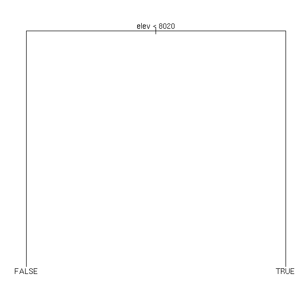
plot(demo.x)
text(demo.x)
demo.x
In comparison to our original tree, this summary also has a list of variables
actually used. In GLM or GAM every variable was used, but in tree classifiers a
variable is only used if it is the best available variable, and especially in
pruned trees many variables never enter the model. In this case, only elev
was used.
node), split, n, deviance, yval, (yprob)
      * denotes terminal node

1) root 160 218.20 FALSE ( 0.5750 0.4250 )
  2) elev < 8020 97  80.07 FALSE ( 0.8557 0.1443 ) *
  3) elev > 8020 63  51.67 TRUE ( 0.1429 0.8571 ) *

summary(demo.x)

Classification tree:
snip.tree(tree = demo, nodes = c(3, 2))
Variables actually used in tree construction:
[1] "elev"
Number of terminal nodes:  2
Residual mean deviance:  0.8338 = 131.7 / 158
Misclassification error rate: 0.1438 = 23 / 160
demo.x <- prune.tree(demo,best=4)
demo.x
node), split, n, deviance, yval, (yprob)
      * denotes terminal node

1) root 160 218.200 FALSE ( 0.57500 0.42500 )
  2) elev < 8020 97  80.070 FALSE ( 0.85567 0.14433 )
    4) slope < 20 89  62.550 FALSE ( 0.88764 0.11236 )
      8) slope < 2.5 35  39.900 FALSE ( 0.74286 0.25714 ) *
      9) slope > 2.5 54   9.959 FALSE ( 0.98148 0.01852 ) *
    5) slope > 20 8  11.090 FALSE ( 0.50000 0.50000 ) *
  3) elev > 8020 63  51.670 TRUE ( 0.14286 0.85714 ) *
summary(demo.x)
Classification tree:
snip.tree(tree = demo, nodes = c(9, 8, 3))
Variables actually used in tree construction:
[1] "elev"  "slope"
Number of terminal nodes:  4
Residual mean deviance:  0.722 = 112.6 / 156
Misclassification error rate: 0.1438 = 23 / 160
Categorical Variables
Just like we did in GLM and GAM, we can use categorical variables in the model
as well. However, instead of having a regression coefficient for all but the
contrast, we try to find the best way to split the categories into two sets. If
a variable has k categories, the number of ways to split it is 2^(k-1) - 1, so
be careful with variables with numerous categories.
demo.2 <- tree(factor(arcpat>0)~elev+slope+pos)
demo.2
node), split, n, deviance, yval, (yprob)
      * denotes terminal node

 1) root 160 220.900 FALSE ( 0.53750 0.46250 )
   2) elev < 7980 96 105.700 FALSE ( 0.76042 0.23958 )
     4) elev < 6930 14   0.000 FALSE ( 1.00000 0.00000 ) *
     5) elev > 6930 82  97.320 FALSE ( 0.71951 0.28049 )
      10) elev < 7460 26  35.890 TRUE ( 0.46154 0.53846 )
        20) pos: ridge,up_slope 12  13.500 FALSE ( 0.75000 0.25000 ) *
        21) pos: bottom,low_slope,mid_slope 14  14.550 TRUE ( 0.21429 0.78571 ) *
      11) elev > 7460 56  49.380 FALSE ( 0.83929 0.16071 )
        22) slope < 2.5 22  28.840 FALSE ( 0.63636 0.36364 )
          44) elev < 7845 12  16.300 TRUE ( 0.41667 0.58333 )
            88) pos: mid_slope,ridge 6   7.638 FALSE ( 0.66667 0.33333 ) *
            89) pos: bottom,low_slope,up_slope 6   5.407 TRUE ( 0.16667 0.83333 ) *
          45) elev > 7845 10   6.502 FALSE ( 0.90000 0.10000 ) *
        23) slope > 2.5 34   9.023 FALSE ( 0.97059 0.02941 )
          46) elev < 7890 24   0.000 FALSE ( 1.00000 0.00000 ) *
          47) elev > 7890 10   6.502 FALSE ( 0.90000 0.10000 ) *
   3) elev > 7980 64  64.600 TRUE ( 0.20312 0.79688 ) *
multi.cv(demo.2)
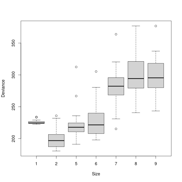
demo2.x <- prune.tree(demo.2,best=5)
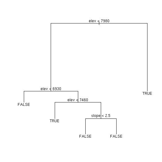
plot(demo2.x)
text(demo2.x)
demo2.x
node), split, n, deviance, yval, (yprob)
      * denotes terminal node

 1) root 160 220.900 FALSE ( 0.53750 0.46250 )
   2) elev < 7980 96 105.700 FALSE ( 0.76042 0.23958 )
     4) elev < 6930 14   0.000 FALSE ( 1.00000 0.00000 ) *
     5) elev > 6930 82  97.320 FALSE ( 0.71951 0.28049 )
      10) elev < 7460 26  35.890 TRUE ( 0.46154 0.53846 ) *
      11) elev > 7460 56  49.380 FALSE ( 0.83929 0.16071 )
        22) slope < 2.5 22  28.840 FALSE ( 0.63636 0.36364 ) *
        23) slope > 2.5 34   9.023 FALSE ( 0.97059 0.02941 ) *
   3) elev > 7980 64  64.600 TRUE ( 0.20312 0.79688 ) *
summary(demo2.x)
Notice how in the pruned tree, pos no longer appears; all the splits
employing pos were pruned off. Notice also that the error rate has
increased significantly for arcpat compared to berrep
(34/160 vs 23/160). Apparently, arcpat has a more complicated
distribution, or responds to variables other than elev and
slope more than does berrep.
Classification tree:
snip.tree(tree = demo.2, nodes = c(23, 22, 10))
Variables actually used in tree construction:
[1] "elev"  "slope"
Number of terminal nodes:  5
Residual mean deviance:  0.8926 = 138.4 / 155
Misclassification error rate: 0.2125 = 34 / 160
Regression Trees
Just as we could use family='poisson' in GLM and GAM models to get
estimates of abundance, rather than presence/absence, we can run the
tree() function in regression mode, rather than classification mode.
We do not have to specify a family argument, however. If the
dependent variable is numeric, tree will automatically produce a
regression tree (this actually trips up quite a few users who have numeric
categories and forget to surround their dependent variable with
factor()).
Now, we'll try and estimate arcpat's abundance with a regression tree.
detach(bryceveg)
attach(cover)
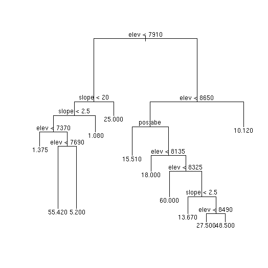
demo.3 <- tree(arcpat~elev+slope+pos)
demo.3
Here, instead of having a list of probabilities of occurrence, the terminal
value at each node is the estimated percent cover of arcpat. For
example, the root node says the overall mean abundance of arcpat is
14.6 percent. This is of course the same value we would get from
node), split, n, deviance, yval
      * denotes terminal node

  1) root 160 101800.0 14.600
    2) elev < 7910 90  33000.0  7.289
      4) slope < 20 83  26870.0  5.795
        8) slope < 2.5 33  22500.0 12.940
         16) elev < 7370 12    203.1  1.375 *
         17) elev > 7370 21  19780.0 19.550
           34) elev < 7690 6   5243.0 55.420 *
           35) elev > 7690 15   3726.0  5.200 *
        9) slope > 2.5 50   1574.0  1.080 *
      5) slope > 20 7   3750.0 25.000 *
    3) elev > 7910 70  57810.0 24.000
      6) elev < 8650 53  48230.0 28.460
       12) pos: bottom,low_slope,up_slope 19  11240.0 15.510 *
       13) pos: mid_slope,ridge 34  32020.0 35.690
         26) elev < 8135 7   6373.0 18.000 *
         27) elev > 8135 27  22890.0 40.280
           54) elev < 8325 8   6000.0 60.000 *
           55) elev > 8325 19  12470.0 31.970
            110) slope < 2.5 6   1710.0 13.670 *
            111) slope > 2.5 13   7820.0 40.420
              222) elev < 8490 5   2938.0 27.500 *
              223) elev > 8490 8   3526.0 48.500 *
      7) elev > 8650 17   5258.0 10.120 *
mean(arcpat)
Following the splits, the first terminal node is 16, where the estimated
abundance of arcpat that has elev < 7370 and slope < 2.5 (collapsing
the tree) is 1.375 percent.
[1] 14.60125
multi.cv(demo.3)
demo3.x <- prune.tree(demo.3,best=11)
summary(demo3.x)
Notice how for a regression tree the summary lists the distribution of residuals,
rather than a classification error rate. The errors are quantitative, exactly as
for a Poisson regression with a GLM or GAM.
Regression tree:
snip.tree(tree = demo.3, nodes = 111)
Number of terminal nodes:  11
Residual mean deviance:  355 = 52900 / 149
Distribution of residuals:
      Min.    1st Qu.     Median       Mean    3rd Qu.       Max.
-6.000e+01 -7.118e+00 -1.080e+00  1.588e-15 -5.626e-01  6.949e+01
Random Forest or randomForest
Random Forest is an algorithm based on classification trees. The idea is to use
"bagging" (bootstrapped permutations of the data) to better estimate the model
and in particular to reduce over-fitting of the model.
Ransom Forest employs a classification tree based on the Gini index, not
deviance, so it's a little different than what we have explored so far. The
particular version we use in R is an appropriation (slighly loaded word) of the
original code by Breiman and Cutler (Breiman 2001), ported to R by Liaw
Wiener (2002) The package is called randomForest (reportedly because
that was the sole permutation of "Random" and "Forest" that Breiman and Cutler didn't
trademark).
The Random Forest algorithm:
Explanatory variable are tracked across replicates to see
which variables reduce the Gini index the most (have the largest effect size).
The final model is an amalgam of the votes of the replicates, and not an actual
single tree.
There are numerous arguments to the randomForest function differing in
defaults for classification versus regression. For our purposes, to fit
a predictive model of presence/absence for
There is no maximum tree size set by default. The algorithm then classifies the
"out-of-bag" samples for each of the 500 trees, pruning back to maximum
cross-validated reduction in the Gini index.
To run the algorithm in R, first load the randomForest package.
library(randomForest) # note the Camelcase
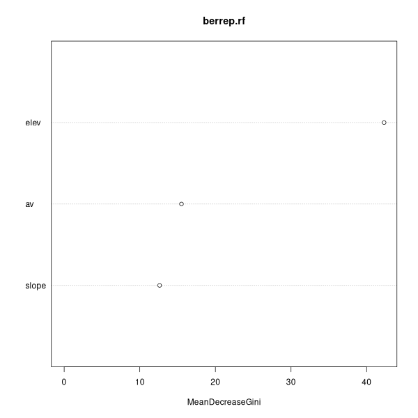
Then, following the above, let's fit a predictive model for presence/absence of
Berberis repens using elevation, aspect value, and slope
berrep.rf <- randomForest(factor(berrep>0) ~ ~ elev + slope + av)
berrep.rf
Call:
randomForest(formula = factor(berrep > 0) ~ elev + slope + av)
Type of random forest: classification
Number of trees: 500
No. of variables tried at each split: 1
OOB estimate of error rate: 15.62%
Confusion matrix:
FALSE TRUE class.error
FALSE 82 10 0.1086957
TRUE 15 53 0.2205882
The default print() function produces a copy of the function call, the
number of trees fitted, the number of variables/tree, the out-of-bag error
estimate, and a confusion matrix. There is no tree to visualize (optionally you
can save all 500 and look at them all keep.forest=TRUE). For a simple
presence/absence model the output is pretty simple, especially if you fit as few
explanatory variables as I did. Nonetheless it's better than we achieved with
the tree classifier (15.62% versus 21.25%). randomForets has a nice
visualization of variable effect size.
varImpPlot(berrep.rf) # note the camelCase
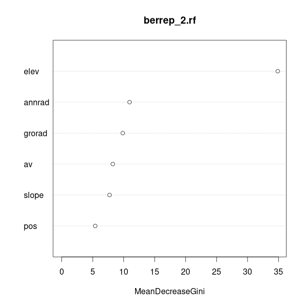
 berrep_2.rf <- randomForest(factor(berrep>0) ~ annrad + av +
elev + grorad + pos + slope)
Surprisingly, the results got worse! Unlike the tree classifier that only
selects variables that help, randomForest() random selects sets of all
variables (in this case of size 2), so some trees are made from poor variables.
To see which variables SHOULD be included, go back to the plot.
berrep_2.rf <- randomForest(factor(berrep>0) ~ annrad + av +
elev + grorad + pos + slope)
Surprisingly, the results got worse! Unlike the tree classifier that only
selects variables that help, randomForest() random selects sets of all
variables (in this case of size 2), so some trees are made from poor variables.
To see which variables SHOULD be included, go back to the plot.
Call:
 randomForest(formula = factor(berrep > 0) ~
               annrad + av + elev + grorad + pos + slope)

               Type of random forest: classification
                     Number of trees: 500
No. of variables tried at each split: 2

        OOB estimate of  error rate: 20.62%
Confusion matrix:
      FALSE TRUE class.error
FALSE    78   14   0.1521739
TRUE 19 49 0.2794118varImpPlot(berrep_2.rf)
 berrep_3_rf <- randomForest(factor(berrep>0) ~
elev + grorad + annrad)
berrep_3_rf
Call:
randomForest(formula = factor(berrep > 0) ~ elev + grorad + annrad)
Type of random forest: classification
Number of trees: 500
No. of variables tried at each split: 1
OOB estimate of error rate: 19.38%
Confusion matrix:
FALSE TRUE class.error
FALSE 76 16 0.1739130
TRUE 15 53 0.2205882
Nope, still slightly worse than our first model.
Like classification trees, randomForest can also be run in regression mode if
the dependent variable is quantitative.
berrep_3_rf <- randomForest(factor(berrep>0) ~
elev + grorad + annrad)
berrep_3_rf
Call:
randomForest(formula = factor(berrep > 0) ~ elev + grorad + annrad)
Type of random forest: classification
Number of trees: 500
No. of variables tried at each split: 1
OOB estimate of error rate: 19.38%
Confusion matrix:
FALSE TRUE class.error
FALSE 76 16 0.1739130
TRUE 15 53 0.2205882
Nope, still slightly worse than our first model.
Like classification trees, randomForest can also be run in regression mode if
the dependent variable is quantitative.
Helpful Functions
multi.cv <- function (tree,n=20)
{
x <- cv.tree(tree)$size
cv <- matrix(0,nrow=n,ncol=length(x))
for (i in 1:n) {
cv[i,] <-rev( cv.tree(tree)$dev)
}
boxplot(cv,names=rev(as.character(x)),
xlab='Size',ylab='Deviance')
}
varImpPlot.tree <- function (tree,progress=FALSE)
{
x <- tree$frame
x$leaf <- as.numeric(row.names(x))
delta <- rep(0,nrow(x))
devs <- rep(0,nlevels(x$var))
names(devs) <- as.character(levels(x$var))
for (i in 1:nrow(x)) {
if (x$var[i] != '
References
Breiman, L. (2001), _Random Forests_, Machine Learning 45(1),
Liaw A., and M. Wiener (2002). Classification and Regression by
randomForest. R News 2(3), 18--22.
5-32.