Generalized Additive Models (GAMs) are designed to capitalize on the strengths of GLMs (ability to fit logistic and poisson regressions) without requiring the problematic steps of a priori estimation of response curve shape or a specific parametric response function. They employ a class of equations called "smoothers" or "scatterplot smoothers" that attempt to generalize data into smooth curves by local fitting to subsections of the data. The design and development of smoothers is a very active area of research in statistics, and a broad array of such functions has been developed. The simplest example that is likely to be familiar to most ecologists is the running average, where you calculate the average value of data in a "window" along some gradient. While the running average is an example of a smoother, it's rather primitive and much more efficient smoothers have been developed.
The idea behind GAMs is to "plot" (conceptually, not literally) the value of the dependent variable along a single independent variable, and then to calculate a smooth curve that goes through the data as well as possible, while being parsimonious. The trick is in the parsimony. It would be possible using a polynomial of high enough order to get a curve that went through every point. It is likely, however, that the curve would "wiggle" excessively, and not represent a parsimonious fit. The approach generally employed with GAMs is to divide the data into some number of sections, using "knots" at the ends of the sections. Then a low order polynomial or spline function is fit to the data in the section, with the added constraint that the derivative of the function at the knots must be the same for both sections sharing that knot. This eliminates kinks in the curve, and ensures that it is smooth and continuous at all points.
The problem with GAMs is that they are simultaneously very simple and extraordinarily complex. The idea is simple; let the data speak, and draw a simple smooth curve through the data. Most ecologists are quite capable of doing this by eye. The problem is determining goodness-of-fit and error terms for a curve fit by eye. GAMs make this unnecessary, and fit the curve algorithmically in a way that allows error terms to be estimated precisely. On the other hand, the algorithm that fits the curve is usually iterative and non-parametric, masking a great deal of complex numerical processing. It's much too complex to address here, but there are at least two significant approaches to solving the GAM parsimony problem, and it is an area of active research.
As a practical matter, we can view GAMs as non-parametric curve fitters that attempt to achieve an optimal compromise between goodness-of-fit and parsimony of the final curve. Similar to GLMs, on species data they operate on deviance, rather than variance, and attempt to achieve the minimal residual deviance on the fewest degrees of freedom. One of the interesting aspects of GAMs is that they can only approximate the appropriate number of degrees of freedom, and that the number of degrees of freedom is often not an integer, but rather a real number with some fractional component. This seems very odd at first, but is actually a fairly straight forward extension of the concepts you are already familiar with. A second order polynomial (or quadratic equation) in a GLM uses two degrees of freedom (plus one for the intercept). A curve that is slightly less regular than a quadratic might require two and a half degrees of freedom (plus one for the intercept), but might fit the data better.
The other aspect of GAMS that is different is that they don't handle interaction well. Rather than fit multiple variables simultaneously, the algorithm fits a smooth curve to each variable and then combines the results additively, thus giving rise to the name "Generalized Additive Models." The point is minimized here, somewhat, in that we never fit interaction terms in our GLMs in the previous lab. For example, it is possible that slope only matters at some range of elevations, giving rise to an interaction of slope and elevation. In practice, interaction terms can be significant, but often require fairly large amounts of data. The Bryce data set is relatively small, and tests of interaction were generally not significant.
The Hastie and Tibshirani version has a slightly broader range of smoothers (including lo() for loess), while Wood's function is restricted to s(). Fortunately, both versions have predict(), fitted(), and most importantly plot() methods. To use the Wood function, download and install package mgcv; to use the Hastie ans Tibshirani function, download and install package gam. Unfortunately, because both functions are named gam() it is awkward to have both packages loaded at the same time.
In my tests, the two implementations are similar but not identical. In addition, there are slight differences in the functions (e.g. default values for arguments). Accordingly, I will present the two implementations separately. You can look at which ever program you use, but I recommend reviewing both to see the effects of the difference in underlying code (Hastie and Tibshirani versus Wood).
To go to the Simon Wood's version, click here
Call: gam(formula = bere > 0 ~ s(elev), family = binomial)
Deviance Residuals:
    Min      1Q  Median      3Q     Max
-2.2252 -0.6604 -0.4280  0.5318  1.9649

(Dispersion Parameter for binomial family taken to be 1)

    Null Deviance: 218.1935 on 159 degrees of freedom
Residual Deviance: 133.4338 on 155 degrees of freedom
AIC: 143.4339

Number of Local Scoring Iterations: 8

DF for Terms and Chi-squares for Nonparametric Effects

            Df Npar Df Npar Chisq  P(Chi)
(Intercept)  1
s(elev)      1       3    18.2882  0.0004
To really see what the results look like, use the plot() function.
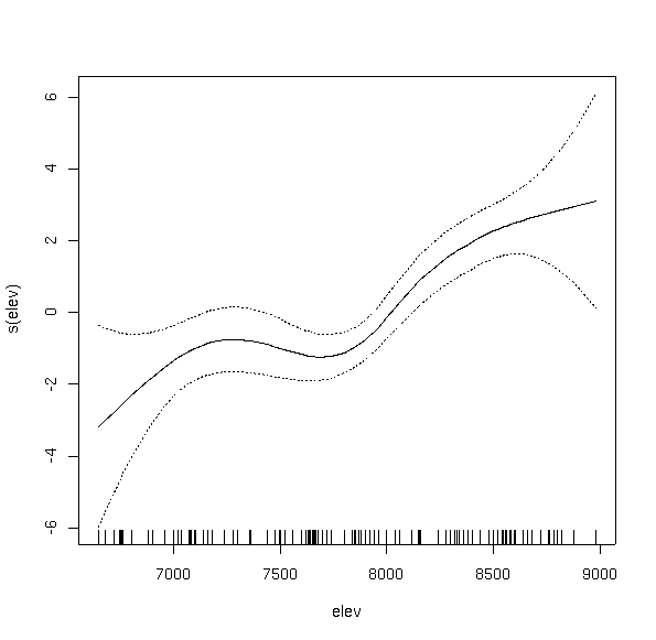
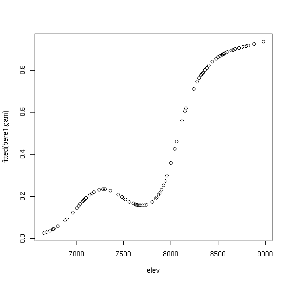
The default plot shows several things. The solid line is the predicted value of the dependent variable as a function of the x axis. The se=TRUE means to plot two times the standard errors of the estimates (in dashed lines). The small lines along the x axis are the "rug", showing the location of the sample plots. The y axis is in the linear units, which in this case is logits, so that the values are centered on 0 (50/50 odds), and extend to both positive and negative values. To see the predicted values on the probability scale we need to use the back transformed values, which are available as fitted(bere1.gam). So,
Notice how the curve has multiple inflection points and modes, even though we did not specify a high order function. This is the beauty and bane of GAMs. In order to fit the data, the function fit a bimodal curve. It seems unlikely ecologically that a species would have a multi-modal response to a single variable. Rather, it would appear to suggest competitive displacement by some other species from 7300 to 8000 feet, or the effects of another variable that interacts strongly over that elevation range.
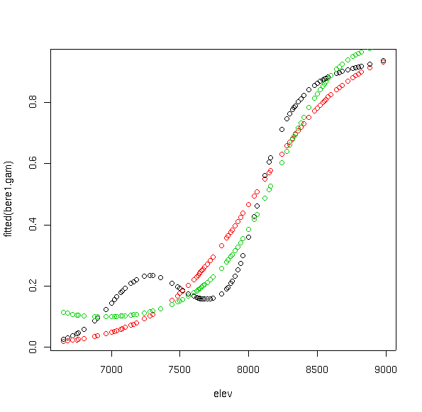
To compare to the GLM fit, we can superimpose the GLM predictions on the plot.
That's the predicted values from the first order logistic GLM in red, and the quadratic GLM in green. Notice how even though the GAM curve is quite flexible, it avoids the problematic upturn at low values shown by the quadratic GLM.
The GAM function achieves a residual deviance of 133.4 on 155 degrees of freedom. The following table gives the comparison to the GLMS.
| model | residual deviance | residual degrees of freedom | |
| GAM | 133.43 | 155 | |
| linear GLM | 151.95 | 158 | |
| quadratic GLM | 146.63 | 157 |
How do we compare the fits? Well, since they're not nested, we can't properly use the anova method from last lab. However, since they're fit to the same data, we can at least heuristically compare the goodness-of-fits and residual degrees of freedom. As I mentioned previously, GAMs often employ fractional degrees of freedom.
Analysis of Deviance Table

Model 1: berrep > 0 ~ elev + I(elev^2)
Model 2: berrep > 0 ~ s(elev)
  Resid. Df Resid. Dev       Df Deviance P(>|Chi|)
1  157.0000    146.627
2  155.0000    133.434   2.0000   13.193     0.001

AIC(bere3.glm,bere1.gam)
          df      AIC
bere3.glm  3 152.6268
bere1.gam  2 143.4339
The GAM clearly achieves lower residual deviance, and at a cost of only two degrees of freedom compared to the quadratic GLM. The probability of achieving a reduction in deviance of 13.2 for 2 degrees of freedom in a NESTED model is about 0.001.
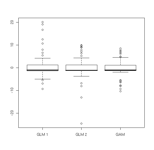
While this probability is not strictly correct for a non-nested test, I think it's safe to say that the GAM is a better fit. In addition, the AIC results are in agreement. One approach to a simple evaluation is to compare the residuals in a boxplot.
boxplot(bere1.glm$residuals,bere3.glm$residuals,bere1.gam$residuals,
    names=c("GLM 1","GLM 2","GAM"))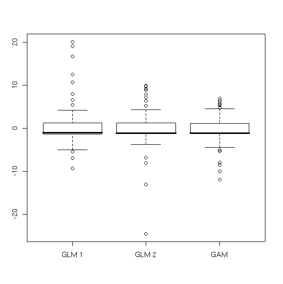
The plot shows that the primary difference among the models is in the number of extreme residuals; the mid-quartiles of all models are very similar.
The interpretation of the slope plot is that Berberis is most likely on midslopes (10-50%), but distinctly less likely on flats or steep slopes. Could a variable with that much error contribute significantly to the fit? Using the anova() function for GAMs, so we can look directly at the influence of slope on the fit.
Analysis of Deviance Table

Model 1: berrep > 0 ~ s(elev) + s(slope)
Model 2: berrep > 0 ~ s(elev)
  Resid. Df Resid. Dev  Df Deviance P(>|Chi|)
1       151    113.479
2       155    133.434  -4  -19.954     0.001
Where before we had a smoothly varying line we now have a scatterplot with some significant departures from the line, especially at low elevations, due to slope effects. As for slope itself
The plot suggests a broad range of values for any specific slope, but there is a modal trend to the data.
Can a third variable help still more. Let's try aspect value (av).
bere3.gam <- gam(berrep>0~s(elev)+s(slope)+s(av),family=binomial)
anova(bere3.gam,bere2.gam,test="Chi")
Analysis of Deviance Table

Model 1: berrep > 0 ~ s(elev) + s(slope) + s(av)
Model 2: berrep > 0 ~ s(elev) + s(slope)
  Resid. Df Resid. Dev       Df Deviance P(>|Chi|)
1  147.0001    100.756
2  151.0000    113.479  -3.9999  -12.723     0.013

AIC(bere3.gam,bere2.gam)
          df      AIC
bere3.gam  4 126.7560
bere2.gam  3 131.4795
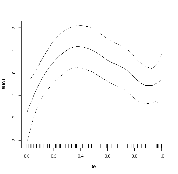
Surprisingly, since aspect value is designed to linearize aspect, the response curve is modal. Berberis appears to prefer warm aspects, but not south slopes. While we might expect some interaction here with elevation (preferring different aspects at different elevations to compensate for temperature), GAMs are not directly useful for interaction terms. Although it's statistically significant, its effect size is small, as demonstrated in the following plot.
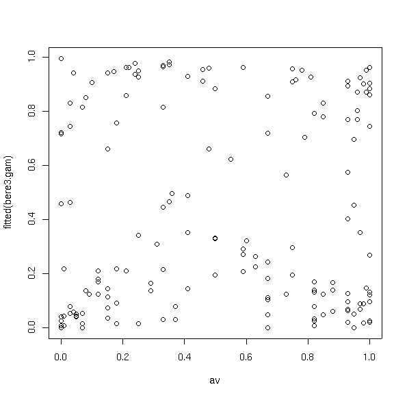
Notice how almost all values are possible at most aspect values. Nonetheless, it is statistically significant.
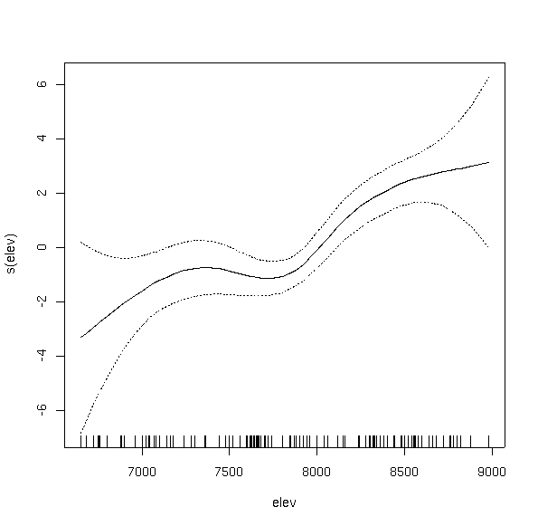
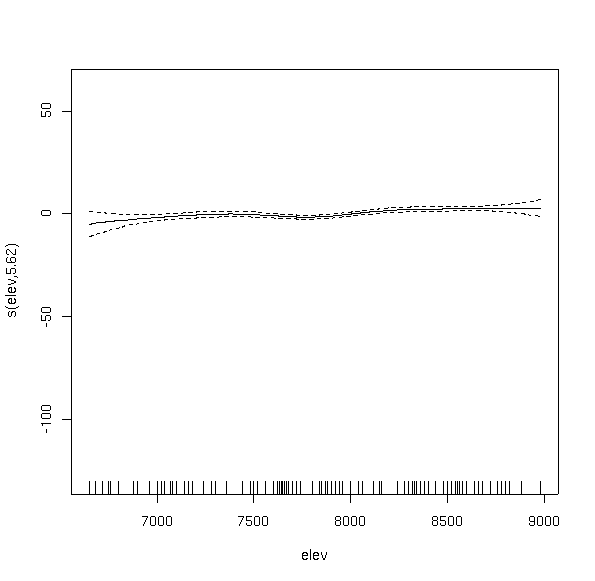
bere1.gam <- gam(bere>0~s(elev),family=binomial)
plot(bere1.gam)
Just as for the GLM, to get a logistic fit as appropriate for presence/absence values we specify family=binomial. The default plot shows several things. The solid line is the predicted value of the dependent variable as a function of the x axis. The dotted lines are plus-or-minus two standard errors, and the small lines along the x axis are the "rug", showing the location of the sample plots. The y axis is in the linear units, which in this case is logits, so that the values are centered on 0 (50/50 odds), and extend to both positive and negative values. To see the predicted values on the probability scale we need to use the back transformed values, which are available as fitted(bere1.gam). So,
Notice how the curve has multiple inflection points and modes, even though we did not specify a high order function. This is the beauty and bane of GAMs. In order to fit the data, the function fit a bimodal curve. It seems unlikely ecologically that a species would have a multi-modal response to a single variable. Rather, it would appear to suggest competitive displacement by some other species from 7200 to 8000 feet, or the effects of another variable that interacts strongly over that elevation range.
To compare to the GLM fit, we can superimpose the GLM predictions on the plot.
points(elev,fitted(bere1.glm),col=2)
points(elev,fitted(bere3.glm),col=3)
That's the predicted values from the first order logistic GLM in red, and the quadratic GLM in green. Notice how even though the GAM curve is quite flexible, it avoids the problematic upturn at low values shown by the quadratic GLM.
How do we compare the fits? Well, since they're not nested, we can't properly use the anova method from last lab. However, since they're fit to the same data, we can at least heuristically compare the goodness-of-fits and residual degrees of freedom. As I mentioned previously, GAMs often employ fractional degrees of freedom. In this case, using the R gam() function, the algorithm achieved a residual deviance of 130.83 and used 4.95 degrees of freedom, stored in bere1.gam$deviance and bere1.gam$edf respectively. The following table gives the respective values.
| model | residual deviance | residual degrees of freedom | |
| GAM | 129.80 | 153.72 | |
| linear GLM | 151.95 | 158 | |
| quadratic GLM | 146.63 | 157 |
The GAM clearly achieves lower residual deviance, and at a cost of 3.28 degrees of freedom compared to the quadratic GLM. The probability of achieving a reduction in deviance of 16.83 for 3.28 degrees of freedom in a NESTED model is about 0.001
Analysis of Deviance Table

Model 1: berrep > 0 ~ elev + I(elev^2)
Model 2: berrep > 0 ~ s(elev)
  Resid. Df Resid. Dev       Df Deviance P(>|Chi|)
1  157.0000    146.627
2  153.7189    129.804   3.2811   16.823     0.001
boxplot(bere1.glm$residuals,bere3.glm$residuals,bere1.gam$residuals,
            names=c("GLM 1","GLM 2","GAM"))
The plot shows that the primary difference among the models is in the number of extreme residuals; the mid-quartiles of all models are very similar.
Warning message:
fitted probabilities numerically 0 or 1 occurred in: gam.fit2(x = args$X,
y = args$y, sp = lsp, S = args$S, rS = args$rS,
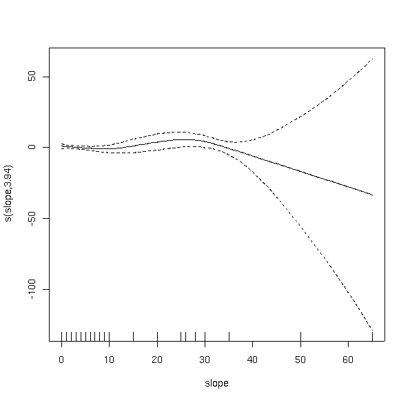
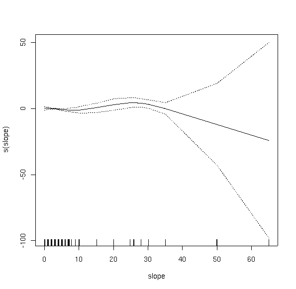
The default is to plot both smooths on the same scale. Accordingly, the result for elevation looks ridiculously flat compared to before (even though it's the same curve) because the standard errors on the smooth of slope are so large.
The interpretation of the slope plot seems to be that Berberis is slightly more likely on moderate slopes (10-30%), but distinctly less likely on steep slopes. Could a variable with that much error contribute significantly to the fit? Since these are nested models we can use anova() to check.
Analysis of Deviance Table

Model 1: berrep > 0 ~ s(elev)
Model 2: berrep > 0 ~ s(elev) + s(slope)
  Resid. Df Resid. Dev       Df Deviance P(>|Chi|)
1  153.7189    129.804
2  149.4435    108.700   4.2753   21.105 0.0003968
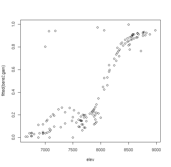
plot(elev,fitted(bere2.gam))
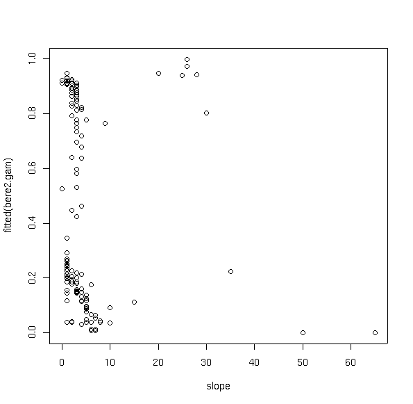
Where before we had a smoothly varying line we now have a scatterplot with some significant departures from the line, especially at low elevations, due to slope effects. As for slope itself
The plot suggests that all possible values obtain at low slopes, where the probabilities are dominated by elevation effects, but that moderate slopes increase the likelihood of Berberis, followed by decreases on steep slopes.
Can a third variable help still more. Let's try aspect value (av).
anova.gam(bere3.gam,bere2.gam,test='Chi')
Analysis of Deviance Table

Model 1: berrep > 0 ~ s(elev) + s(slope) + s(av)
Model 2: berrep > 0 ~ s(elev) + s(slope)
  Resid. Df Resid. Dev       Df Deviance P(>|Chi|)
1  144.8843     95.407
2  149.4435    108.700  -4.5593  -13.293     0.015
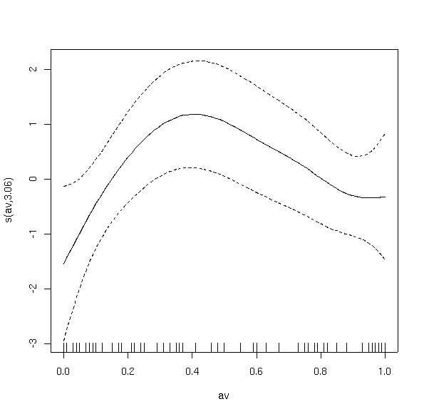
Surprisingly, since aspect value is designed to linearize aspect, the response curve is modal. Berberis appears to prefer east and west slopes to north or south. While we might expect some interaction here with elevation (preferring different aspects at different elevations to compensate for temperature), GAMs are not directly useful for interaction terms. Although it's statistically significant, its effect size is small, as demonstrated in the following plot.
Notice how almost all values are possible at most aspect values. Nonetheless, there is a small modal trend.
My own feeling is that given the ease of creating and presenting graphical output, the increased goodness-of-fit of GAMs and the insights available from analysis of their curvature over sub-regions of the data make GAMs a superior tool in the analysis of ecological data. Certainly, you can argue either way.
Like GLMs, they are suitable for fitting logistic and poisson regressions, which is of course very useful in ecological analysis.
Wood, S.N. (2000) Modelling and Smoothing Parameter Estimation with Multiple Quadratic Penalties. J.R.Statist.Soc.B 62(2):413-428
Wood, S.N. (2003) Thin plate regression splines. J.R.Statist.Soc.B 65(1):95-114
Wood, S.N. (2004a) Stable and efficient multiple smoothing parameter estimation for generalized additive models. J. Amer. Statist. Ass. 99:673-686
Wood, S.N. (2004b) On confidence intervals for GAMs based on penalized regression splines. Technical Report 04-12 Department of Statistics, University of Glasgow.
Wood, S.N. (2004c) Low rank scale invariant tensor product smooths for generalized additive mixed models. Technical Report 04-13 Department of Statistics, University of Glasgow.