Fortunately, alternative inferential statistics have been developed which eliminate (or at least finesse) these problems. The first technique we will explore is "Generalized Linear Models", specifically techniques known as "logistic regression" and "poisson regression."
Suppose we had two vectors:
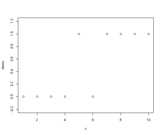
demo <- c(0,0,0,0,1,0,1,1,1,1)
x <- 1:10
Suppose we try fitting a linear regression through these data.
demo.lm <- lm(demo~x)
summary(demo.lm)
Call:
lm(formula = demo ~ x)

Residuals:
       Min         1Q     Median         3Q        Max
-5.697e-01 -1.455e-01 -3.469e-18  1.455e-01  5.697e-01

Coefficients:
            Estimate Std. Error t value Pr(>|t|)
(Intercept) -0.26667    0.22874  -1.166  0.27728
x            0.13939    0.03687   3.781  0.00538 **
---
Signif. codes:  0 `***' 0.001 `**' 0.01 `*' 0.05 `.' 0.1 ` ' 1

Residual standard error: 0.3348 on 8 degrees of freedom
Multiple R-Squared: 0.6412,     Adjusted R-squared: 0.5964
F-statistic:  14.3 on 1 and 8 DF,  p-value: 0.005379
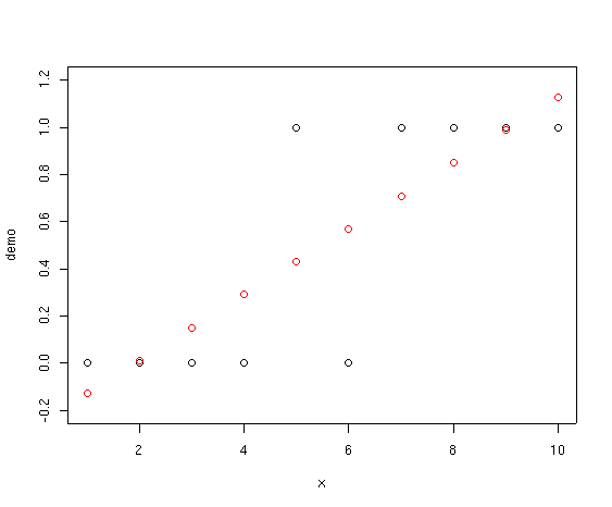
Notice how the fitted points start below 0 and slant upward past 1.0. If we
interpret these values as probabilities that species
Actually, there are two primary problems:
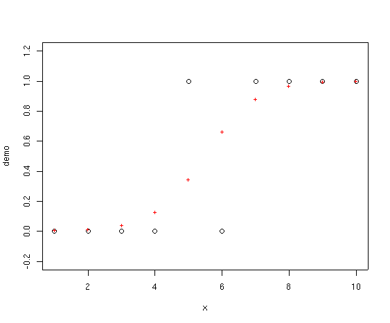
Alternatively, we can fit a generalized linear model that models the log of the
odds (called the logit) rather than the probability, and finesse both problems
simultaneously. If we fit a GLM as follows
The red crosses represent the fitted values from the GLM. Notice how they never
go below 0.0 or above 1.0. In addition, the family=binomial
specification in the glm() function specifies a logistic regression
and makes sure that the fitting
function knows that the variance is proportional to the fitted value times 1
minus the
fitted value, rather
than constant.
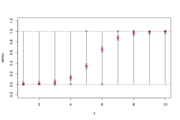
OK, so where does deviance enter in? Deviance is calculated as -2 * the
log-likelihood. In a logistic regression you can visualize the deviance as
lines drawn from the fitted point to 0 and 1, as shown below.
We take the length of each arrow and multiply that times the log of that
length and add to the same calculation for the other arrow for that point.
Finally, take -2 * the sum of all those values. If you look at the first
point, for example, the fitted value is almost exactly on top of the
actual value, so the length of one of the arrows is almost zero (and in fact not
shown on the drawing as they are too small to draw). For this point, the
deviance is very small. In fact
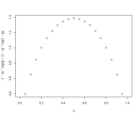
What's the most deviance a single point can contribute? Well, let's
look at the distribution for deviance for all probabilities between 0 and 1.
Notice how the curve is uni-modal, symmetric, and achieves its maximum value at
0.5. Notice too how probabilities greater than 0.2 and less than 0.8 have deviance
greater than 1. The maximum deviance for a single point in a logistic regression
is for probability = 0.5, where it reaches 1.386294.
First, get into the appropriate directory for the Bryce data, and start R.
Then, remember to attach both site and
veg.
To model the presence/absence of Berberis as a function of elevation, we use:
bere1.glm<-glm evaluates to "store the result of the generalized linear
model
in an object called 'bere1.glm'." Any object name could be used, but
"variable.glm"
is concise and self-explanatory. The number 1 is in anticipation of fitting
more models later.
berrep>0 evaluates to a logical, 0 (absent) or 1 (true), and ~
elev evaluates to "as a function of elevation." The family =
binomial tells R to perform logistic regression, as opposed to other
forms of GLM.
R calls the estimated probabilities "fitted values", and we
can use the fitted function to extract the probabilities from our GLM
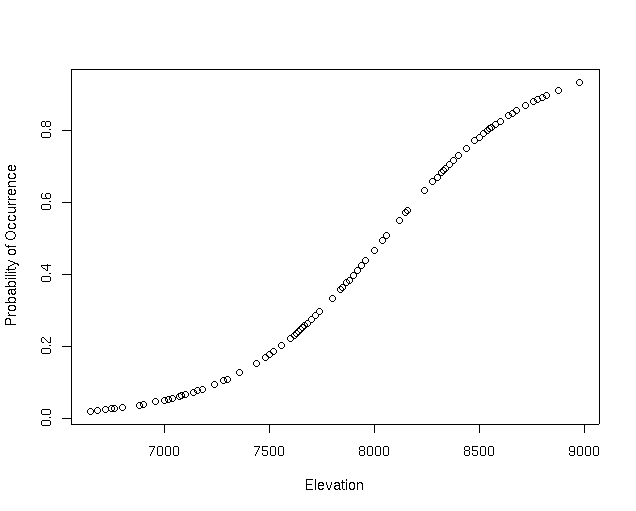
object (bere1.glm). To see a graphical representation of the fitted model, do
Notice how the fitted curve is a smooth sigmoidal curve. The logistic
regression is linear in the logit, but when back transformed from the
logit to probabilities, it's sigmoidal. This is a good start, but we originally
assumed that the presence/absence of Berberis was a function of both
elevation and aspect. In addition, following conventional ecological theory we
might assume that the probability exhibits a unimodal response to environment.
To get a smooth unimodal response is simple. Just as a linear logistic
regression is sigmoidal when back transformed to probability, a quadratic
logistic regression is unimodal symmetric when back transformed to
probabilities. Accordingly, let's fit a model that is quadratic for elevation
and aspect value. We use:
~elev+I(elev^2)+av+I(av^2) evaluates to "as a function of elevation, elevation squared,
aspect value, and aspect value squared." The I(elev^2) tells R
that "I really do mean elevation squared" so that it doesn't attempt to
interpret the ^2 as an R formula operator. If you forget and
type elev+elev^2 R will mis-interpret your intent.
All together, bere2.glm<-glm(berrep>0~elev+I(elev^2)+av+I(av^2),family=binomial) models
the probability of the presence of Berberis as a unimodal function of elevation and
aspect value.
The details of the object are available with the summary function.
The output includes a Z statistic
(standardized normal deviate) and p value for each variable in the model, and tests the
hypothesis that the true value of each coefficient is 0. As you can determine
from the output, it appears that elev and I(elev^2) are
significantly different from 0, and the intercept is marginal.
While glm models do not have quite the same properties as
ordinary least squares (e.g. deviance instead of variance), you can still
get good indications about the performance of the model. Analogous to
R^2, 1-(residual deviance/null deviance) is a good indicator of overall
model fit. E.g.
The test being performed assumes
that the difference in deviance (See Deviance column) attributed to a
particular variable is distributed as Chi-square with the number of degrees of
freedom attributed to that variable (See Df column). E.g., the
elev variable achieves a reduction in deviance of 66.247 at a cost of 1
degree of freedom; the associated probability of that much reduction by chance
(Type I error) is essentially 0. It is important to realize that this table
uses the variables in the order given in the equation, and that each variable is
tested against the residual deviance after earlier variables (including the
intercept) have been taken into account.
The indication is that elevation is very important, and that the quadratic
term is also statistically significant. Neither av nor I(av^2) is significant,
at least after accounting for elevation.
For nested models (where a simpler model is a formal subset of the more complex
model) it is also possible to compare glms with the anova function as follows:
Alternatively, we can compare the AIC values for the two models with the
AIC() function. Here, we choose the model with the smaller AIC as
superior. The output is much more terse, and we have to remember which terms
are in each model.
The analysis suggests that addition of av and av^2 is not a significant
improvement, as we determined before.
So, how good is the model? For the time being (and for the sake of
demonstration), we're going to stick with our full model even though we don't
believe av matters. We'll delete it later and see the results.
Our pseudo-R^2 of 0.34 suggests that the model is
not great, but plant species are often difficult to model well, and we've just
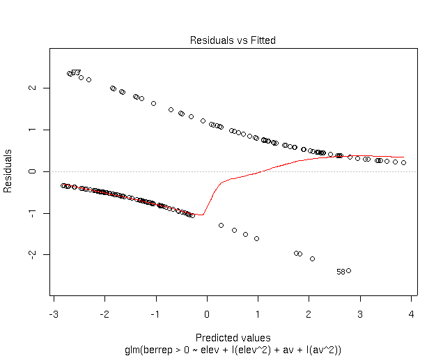
started. To evaluate the model more fully, let's look at graphic output.
As you can see, the residuals occur in two curves; the upper one corresponds to
plots where Berberis occurs, and the lower to absence sites. The X and Y axes
are in logits (log of the odds), rather than probabilities, because that's the
scale that the model (and thus the residuals) is fit on.
Note that
the density of points is higher on the upper curve for fitted values
> 0.75, with residuals approaching 0. Similarly, the density of points
on the lower curve is higher at fitted values
< 0.3, again with residuals near 0. So, sites where Berberis is
present mostly have high fitted values, meaning that the model would predict
Berberis there. Unfortunately, Berberis also occurs on sites with
fitted values approaching 0, meaning that Berberis is definitely not
predicted at those sites; those are errors. Mostly, however, where Berberis is
absent, we predict absence.
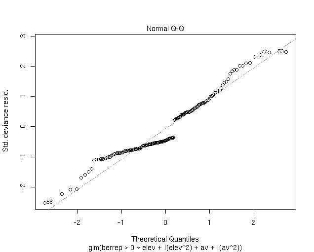
The second plot shows the ordered residuals compared to a normal distribution.
If the residuals are approximately normally distributed we can have more faith
in the robustness of the model. In this case, our extreme residuals are more
extreme than a normal distribution, but that's not uncommon for GLM models.
As an alternative, we can calculate the fraction (or equivalently, percent) of plots
correctly predicted with the table function. Since R refers to
the estimated probabilities as fitted values, we can use the fitted
function to extract the fitted values and do the following:
That's all well and good, but what does our model really look like? Well, the
current model is multi-dimensional for elev and av, so it's
problematic to look at directly.
In this case we can look at the model
one dimension at a time.
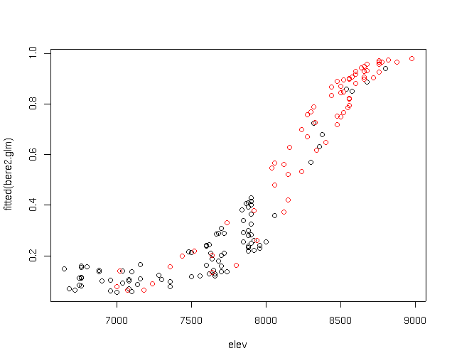
Notice how the points make a fairly smooth curve as elevation increases; this
is the effect due to elevation. Notice also that there is a small vertical
distribution of points at any given elevation; this is the effect due to aspect
value. Notice also that the thickness of the band due to aspect value is about
0.2 at its maximum, while the amplitude of the elevation curve goes from about
0.1 to 1.0. This is a crude estimate of "effect size", where elevation has more
than 5 times the effect than aspect value on the predicted value. We can make
more precise estimates later, but graphic intuition is always nice, and we don't
have to learn any more R to see it. The points command above
colors those plots where Berberis actually occurs, so we again get a
sense of how well the model is doing.
As we noted before, the av and I(av^2) variables are not
contributing significantly to the fit. If we look at the model without them, we get:
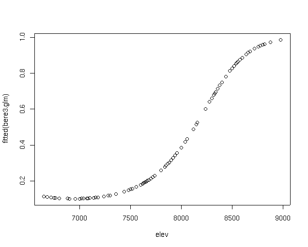
Notice how the scatter due to av is now gone, and we get a clear picture of
the relationship of the probability of Berberis to elevation. Notice too
that the curve actually goes up slightly at lower elevations; this is
unexpected and probably ecologically improbable given what we know about species
response to environment. While it first appeared that the GLM was successful in
fitting a modal response model to the elevation data, what we actually observe is a
truncated portion of an inverted modal curve. If you go back and look at the
coefficients fit by the model, you see:
In fact, converted to a simple
test, the simple GLM has equal prediction accuracy (0.85).
As another example of nested calls,
we can plot the linear model without storing it as follows:
The analysis added soil depth to the existing model. The notation
update(bere.glm,.~.+depth means update model bere.glm, use the
same formula, but add depth. The na.action=na.omit means omit
cases where soil depth is unknown. Unfortunately, several plots in the data set
don't have soil data.
As you should recall from Lab 2, soil depth and elevation were not independent,
with deeper soils generally occurring at lower elevations. This last model
suggests that soil depth is significant, even after accounting for elevation.
We actually observe slightly higher deviance reduction due to elevation than
before, but this is due to dropping those plots where soil depth is unknown, not
to a change in the effect of elevation.
Variables can be dropped as well, as for example:
We can calculate a number of statistics on the cells of the table. Among the
more commonly employed are
This is actually a tricky model to fit. If none of the observed or expected values actually
approach 100.0, we can treat the distribution as bounded at 0 on the low end,
and unbounded on the upper. In this case, the best choice might be a Poisson
distribution, where we treat the percent cover as equivalent to numbers of
individuals, ramets, or modules.
In Poisson regression we are again working with deviance, as opposed to
variance, but the deviance is calculated differently.
$$d = 2 \times \sum_{i-1}^N y_i \times log(y_i/\hat y_i) - (y_i - \hat y_i)$$
where \(y_i\) is the abundance of the species in sample unit \(i\) and \(\hat
y_i\) is the fitted value. Once again, I'll use a simplistic example to
demonstrate.
In real analyses we run into the complication that some values of abundance are
zero, and \(log(0)\) is undefined, so
$$ log(0/\hat y_i)$$
is also undefined. In this case since \(y_i\) is 0, 0 times anything is zero,
and we simply drop out the term
$$y_i \times log(y_i/\hat y_i)$$
That leaves \(- (y_i - \hat y_i) = \hat y_i\).
Back in Lab 1 we created a dataframe called cover which had the cover
class midpoints instead of cover codes. Using this, let's model the expected
abundance of Berberis repens. The most important change we will make in
the function call is to specify a new family. For a Poisson
distribution the variance is proportional to the mean, and we can specify that
with family='poisson' in our function call, instead of
family='binomial'. A second, trivial change is to round the percent
cover to integer values, as a Poisson distribution expects counts. An
alternative is to use ceiling() instead of round, which converts real
numbers to the smallest integer that is larger than the number. In our case,
round(0.5) = 0 while ceiling(0.5) = 1.
Often the distributions of plant species are difficult to model due to extreme
values in the distribution. As an example of a contrast, let's try
Arctostaphylos patula.
Allouche, O., A. Tsoar and R. Kadmon. 2006. Assessing the accuracy of species
distribution models: Prevalence, kappa and the True Skill Statistic (TSS).
Journal of Applied Ecology 43(6):1223--1232.
Huisman, J., H. Olff, and L.F.M. Fresco. 1993. A hierarchical set of models for
species response analysis. Journal of Vegetation Science, 4, 37-46.
Cohen, J. 1960. Coefficient of agreement for nominal scales. Educational
Psychology 20:37--40.
ter Braak, C.J.F. and C.W.N. Looman. 1995. Regression. Pages 39-77 IN
R.H.G. Jongman, C.J.F. ter Braak, and O.F.R. Van Tongeren. (eds.) Data
analysis in community and landscape ecology. Cambridge University Press.
we get
demo.glm <- glm(demo~x,family=binomial)
plot(x,demo,ylim=c(-0.2,1.2))
points(x,fitted(demo.glm),col=2,pch="+")
 fitted(demo.glm)
shows that the fitted value of the first point is 0.002850596. If we calculate the deviance for just that point
fitted(demo.glm)
shows that the fitted value of the first point is 0.002850596. If we calculate the deviance for just that point
          1           2           3           4           5           6
0.002850596 0.010397540 0.037179991 0.124285645 0.342804967 0.657195033
          7           8           9          10
0.875714355 0.962820009 0.989602460 0.997149404
-2 * (0.002850596*log(0.002850596)+(1-0.002850596)*log(1-0.002850596))
[1] 0.03910334
it's only 0.03910334, a very small value. If we look at point 5, its fitted
values is 0.342804967. The deviance associated with point 5 is
-2 * (0.342804967*log(0.342804967)+(1-0.342804967)*log(1-0.342804967))
[1] 1.285757
This is a much higher value. In a logistic regression, deviances
of greater than one for a single point are indicative of poor fits.
q <- seq(0.0,1.0,0.05)
plot(q,-2*(q*log(q)+(1-q)*log(1-q)))
Examples with the Use of R
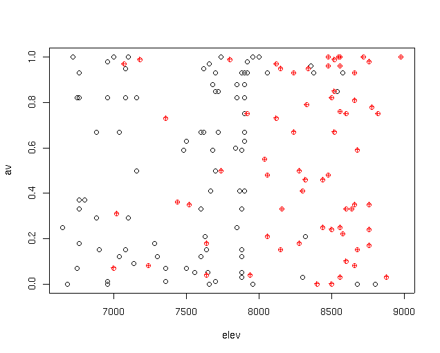
Returning to the Bryce Canyon data set, we will attempt to model the distribution
of Berberis (Mahonia) repens, a common shrub in mesic portions of Bryce Canyon.
Preliminary
graphical analysis (shown below, Berberis locations in red)
suggests that the distribution of Berberis
repens is related to elevation and possibly aspect value.
 bere1.glm <- glm (berrep>0 ~ elev, family = binomial)
Remember that in R equations are given in a general form, and that
we can use logical subscripts.
bere1.glm <- glm (berrep>0 ~ elev, family = binomial)
Remember that in R equations are given in a general form, and that
we can use logical subscripts.
plot(elev,fitted(bere1.glm),xlab='Elevation',
             ylab='Probability of Occurrence')
 bere2.glm <- glm(berrep>0~elev+I(elev^2)+av+I(av^2),family=binomial)
summary(bere2.glm)
The listing includes deviance residuals quartiles, variable coefficients,
null deviance vs residual deviance,
and
an AIC (Akaike information criterion) statistic. This last item doesn't concern us yet,
but will be handy later on.
bere2.glm <- glm(berrep>0~elev+I(elev^2)+av+I(av^2),family=binomial)
summary(bere2.glm)
The listing includes deviance residuals quartiles, variable coefficients,
null deviance vs residual deviance,
and
an AIC (Akaike information criterion) statistic. This last item doesn't concern us yet,
but will be handy later on.
Call:
glm(formula = berrep > 0 ~ elev + I(elev^2) + av + I(av^2),
                  family = binomial)

Deviance Residuals:
    Min       1Q   Median       3Q      Max
-2.3801  -0.7023  -0.4327   0.5832   2.3540

Coefficients:
              Estimate Std. Error z value Pr(>|z|)
(Intercept)  7.831e+01  4.016e+01   1.950   0.0512 .
elev        -2.324e-02  1.039e-02  -2.236   0.0254 *
I(elev^2)    1.665e-06  6.695e-07   2.487   0.0129 *
av           4.385e+00  2.610e+00   1.680   0.0929 .
I(av^2)     -4.447e+00  2.471e+00  -1.799   0.0719 .
---
Signif. codes:  0 '***' 0.001 '**' 0.01 '*' 0.05 '.' 0.1 ' ' 1

(Dispersion parameter for binomial family taken to be 1)

    Null deviance: 218.19  on 159  degrees of freedom
Residual deviance: 143.19  on 155  degrees of freedom
AIC: 153.19

Number of Fisher Scoring iterations: 5
1-(143.1878/218.1935)
[1] 0.3437577
In addition, each term term in the model can be tested in
several ways. In order, they can be tested with the anova function,
particularly with a Chi-square test statistic.
anova(bere2.glm,test="Chi")
Analysis of Deviance Table

Model: binomial, link: logit

Response: berrep > 0

Terms added sequentially (first to last)


           Df Deviance Resid. Df Resid. Dev P(>|Chi|)
NULL                         159    218.193
elev        1   66.247       158    151.947 3.979e-16
I(elev^2)   1    5.320       157    146.627     0.021
av          1    0.090       156    146.537     0.765
I(av^2)     1    3.349       155    143.188     0.067
bere3.glm<-glm(berrep>0~elev+I(elev^2),family=binomial)
anova(bere3.glm,bere2.glm,test="Chi")
The table is telling us that the reduction in deviance attributable to adding
av and I(av) is 3.439, and that the probability of getting
that with an additional 2 degrees of freedom is 0.179. This suggests strongly
that aspect value is not significant.
Analysis of Deviance Table

Model 1: berrep > 0 ~ elev + I(elev^2)
Model 2: berrep > 0 ~ elev + I(elev^2) + av + I(av^2)
  Resid. Df Resid. Dev  Df Deviance P(>|Chi|)
1       157    146.627
2       155    143.188   2    3.439     0.179
AIC(bere2.glm,bere3.glm)
          df      AIC
bere2.glm  5 153.1878
bere3.glm  3 152.6268
plot(bere2.glm)
R gives you four plots
(waiting for a carriage return before plotting the next panels). What we're
interested in is a plot of the residuals of the model. However, if you're used
to looking at residuals of linear regression plots, you're bound to find the
residual plots of logistic GLM odd (or possibly depressing). Because the only
possible values to the actual data are 0 or 1, many of the residuals are
necessarily large, and show an interesting trend.
plot(bere2.glm)
Hit Return to see next plot:
 table(berrep>0,fitted(bere1.glm)>0.5)
This is slightly complicated, so let's look at the call. berrep>0 you
remember evaluates to a logical (TRUE or FALSE); fitted(bere1.glm)>0.5 does the
same for the estimated probabilities. Here, however, we want to classify all
plots with a probability > 0.5 as "present" (or in this case TRUE), and those
less than 0.5 as 0 or FALSE.
The first variable in the call is listed as the rows, and the second variable as
the columns. As you can see, we correctly predicted 136 out of 160 plots
(0.85). In addition, we made slightly fewer "errors of commission" (predicted
Berberis to be present when it's absent = 9) than "errors of omission"
(predicted absent when present = 15 ). These errors can be seen on the first
residual plot as well. Overall, our model is fair, but is biased, and
under-predicts Berberis slightly.
table(berrep>0,fitted(bere1.glm)>0.5)
This is slightly complicated, so let's look at the call. berrep>0 you
remember evaluates to a logical (TRUE or FALSE); fitted(bere1.glm)>0.5 does the
same for the estimated probabilities. Here, however, we want to classify all
plots with a probability > 0.5 as "present" (or in this case TRUE), and those
less than 0.5 as 0 or FALSE.
The first variable in the call is listed as the rows, and the second variable as
the columns. As you can see, we correctly predicted 136 out of 160 plots
(0.85). In addition, we made slightly fewer "errors of commission" (predicted
Berberis to be present when it's absent = 9) than "errors of omission"
(predicted absent when present = 15 ). These errors can be seen on the first
residual plot as well. Overall, our model is fair, but is biased, and
under-predicts Berberis slightly.
        FALSE TRUE
  FALSE    83    9
  TRUE     15   53
plot(elev,fitted(bere2.glm))
points(elev[berrep>0],fitted(bere2.glm)[berrep>0],col=2)
 plot(elev,fitted(bere3.glm))
 What's important here is that the linear term elev is negative, while
the quadratic term I(elev^2) is positive. This is indicative of an
inverted fit; what we want is a positive linear term and negative quadratic term
to get a classical unimodal response curve. Some ecologists (e.g. ter Braak and Looman
[1995]) suggest that inverted curves should not be accepted, as they violate our
ecological understanding and are dangerous if extrapolated. On the other hand,
if accurate prediction is the primary objective, we might prefer an "improper"
fit if it is more accurate within the range of our data. We can test for this,
of course, as follows:
What's important here is that the linear term elev is negative, while
the quadratic term I(elev^2) is positive. This is indicative of an
inverted fit; what we want is a positive linear term and negative quadratic term
to get a classical unimodal response curve. Some ecologists (e.g. ter Braak and Looman
[1995]) suggest that inverted curves should not be accepted, as they violate our
ecological understanding and are dangerous if extrapolated. On the other hand,
if accurate prediction is the primary objective, we might prefer an "improper"
fit if it is more accurate within the range of our data. We can test for this,
of course, as follows:
elev        -2.323e-02  1.030e-02  -2.256   0.0241 *
I(elev^2)    1.664e-06  6.631e-07   2.510   0.0121 *
anova(bere3.glm,glm(berrep>0~elev,family=binomial),test="Chi")
In this case I didn't even store the linear logistic equation, I simply embedded
the call to glm within the anova function. (Actually, we
already calculated this model as bere1.glm, but I wanted to demonstrate nested
calls for future use). As you
can see,
the quadratic term achieves a small but significant reduction in deviance.
The AIC analysis agrees.
Analysis of Deviance Table

Response: berrep > 0


                 Resid. Df Resid. Dev  Df Deviance P(>|Chi|)
elev + I(elev^2)       157    146.627
elev                   158    151.947  -1   -5.320     0.021
AIC(bere3.glm,glm(berrep>0~elev,family=binomial))
If we decide not to accept the inverted modal GLM, going back to the simpler
model would only be slightly less accurate.
                                          df      AIC
bere3.glm                                  3 152.6268
glm(berrep > 0 ~ elev, family = binomial)  2 155.9469
table(berrep>0,fitted(bere1.glm)>0.5)
This is
an example where minimizing deviance and maximizing prediction accuracy are not
the same thing. Some statistical approaches let you choose the criterion to
optimize, but GLM does not, at least directly.
      FALSE TRUE
FALSE    83    9
 TRUE    15   53
plot(elev,fitted(glm(berrep>0~elev,family=binomial)))
Models can be modified by adding or dropping specific terms, with an abbreviated
formula as follows:
bere4.glm<-update(bere2.glm,.~.+depth,na.action=na.omit)
anova(bere4.glm,test="Chi")
Analysis of Deviance Table

Model: binomial, link: logit

Response: berrep > 0

Terms added sequentially (first to last)


           Df Deviance Resid. Df Resid. Dev P(>|Chi|)
NULL                         144    197.961
elev        1   69.702       143    128.258 6.896e-17
I(elev^2)   1    2.677       142    125.581     0.102
av          1    0.080       141    125.502     0.778
I(av^2)     1    7.592       140    117.910     0.006
depth       1   12.422       139    105.488 4.243e-04
bere5.glm<-update(bere2.glm,.~.-av-I(av^2))
summary(bere5.glm)
Note, however, that I had to use the I(av^2) instead of the simpler
av^2 to get the correct result.
Generalized linear models are an enormously powerful tool for the analysis of
the distribution of plant species along environmental gradients. A
variant of this approach using principles of parsimony has been advocated by
Huisman, Olff and Fresco (1993). They proposed testing a series of
increasingly more complicated models from a flat null model to a skewed
(non-symmetric) curve for individual species. However, their models are not
easily fit by the maximum likelihood methods of GLM, and require non-linear
regression by least squares (although see the HOF
models of Jari Oksanen for a maximum likelihood approach).
Call:
glm(formula = berrep > 0 ~ elev + I(elev^2), family = binomial)

Deviance Residuals:
    Min       1Q   Median       3Q      Max
-2.5304  -0.6914  -0.4661   0.5889   2.1420

Coefficients:
              Estimate Std. Error z value Pr(>|z|)
(Intercept)  7.310e+01  3.979e+01   1.837   0.0662 .
elev        -2.167e-02  1.027e-02  -2.110   0.0349 *
I(elev^2)    1.560e-06  6.613e-07   2.359   0.0183 *
---
Signif. codes:  0 '***' 0.001 '**' 0.01 '*' 0.05 '.' 0.1 ' ' 1

(Dispersion parameter for binomial family taken to be 1)

    Null deviance: 218.19  on 159  degrees of freedom
Residual deviance: 146.63  on 157  degrees of freedom
AIC: 152.63

Number of Fisher Scoring iterations: 4
Predictive Model
It is often the case that we want to use our logistic regression model to develop a map of
predicted habitat. To do this, typically we convert the model to a threshold
that converts all fitted values above the threshold to PRESENT and all fitted
values below the threshold to ABSENT. The values of predicted present or
absent can then be compoared to observed present or absent in a two-by-two
contingency table. Unlike the example given above, the table is typically
strured so that TRUE is the first row and column, and FALSE is the second row
and colum as shown below.

Prevalence \(P\) \(a+c\) Predicted Prevalence \(P^\prime\) \(a + b\) Sensitivity \(Se\) \(a/(a+c)\) Specificity \(Sp\) \(d/(b+d)\) Positive Predictive Power \(PPP\) \(a/(a+b)\) Cohen's \(\kappa\)
Cohen's \(\kappa\) is a widely used index of agreement for \(2\times 2\) contingency
tables. \(\kappa\) is designed to correct for the fraction of agreement between
two assessments expected by chance (Cohen 1960), thus identifying the
marginal increase in agreement due to model fit and the choice of threshold.
The \(\kappa\) statistic has equation
$$
\kappa = \frac{(a+d)/N - x}{1 - x}
$$
where the expected agreement by chance is given by
$$
x = \bigl((a+b) \times (a+c) + (d+c) \times (d+b)\bigr)/N^2
$$
Using \(\kappa\), the threshold is selected to maximize \(\kappa\).
The True Skill Statistic (TSS)
More recently, \(\kappa\) has been largely superseded by the True Skill Statistic
(TSS) (Allouche et al. 2006).
$$
TSS = \frac{ad - bc}{(a+c) \times (b+d)} = \frac{a}{a + c} + \frac{d}{b + d}
- 1 = \frac{1}{a+c} - \frac{b}{b+d}
$$
TSS is commonly given as the sum of `sensitivity' and `specificity'
minus 1
where
$$
TSS = Se + Sp - 1;\qquad Se = \frac{a}{a + c} \quad {\rm and} \quad Sp =
\frac{d}{b + d}
$$
as given in the second form just above. Like \(\kappa\), the threshold
is chosen to maximize TSS.
Obviously, the values pf \(a, b, c\) and \(d\) depend on where you set the
threshold between PRESENT and ABSENT, and the problem is to choose the
appropriate probability to maximize \(\kappa\) or TSS. The algorithm I
recommend is to sort the observed values in the order of their probability from
high to low, and
then sort the probabilities from high to low as well. Then, iteratively set the threshold
at each point and calculate \(\kappa\) and TSS. Plotting the distributions of
various table statistics as well as \(\kappa\) and TSS allows visualization of
the behavior of the stats. It's then a simple matter of choosing the
probability that maximizes \(\kappa\) or TSS. A function called
Mttthresh(brycecveg$berrep>0,fitted(bere3.glm)
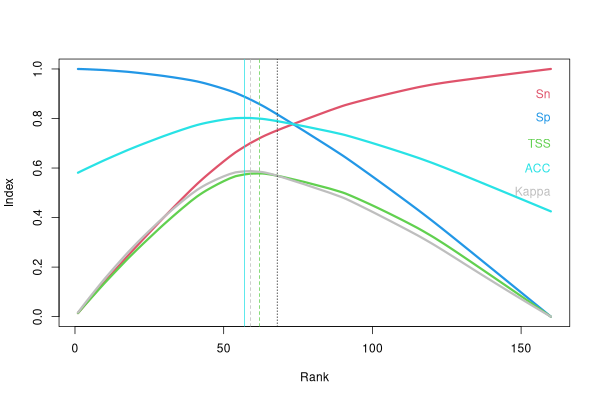
      rank      pval     value        a        b        c        d
kappa   59 0.4879088 0.5875453 47.65143 11.34857 20.34857 80.65143
TSS     62 0.4348241 0.5781561 48.95590 13.04410 19.04410 78.95590
ACC     57 0.5156818 0.8021951 46.67561 10.32439 21.32439 81.67561
In this case the suggested probabilities are not far off from 0,5, but that is
not necessarily true in general. ACC is accuracy, so we're at about 0.8 correct
predictions.
Poisson Regression
In all the above regressions, we have modeled the probability of the presence of
Berberis repens. If we want to model the expected abundance of Berberis repens
we can still use GLM, but we need to specify the model slightly differently. As you will recall,
the two elements of GLM were to finesse the boundedness problem of the dependent variable, and to
use the appropriate variance for the estimated values. If we want to model expected abundance in percent cover,
it is again bounded at the lower limit at 0.0, but is now bounded at the upper end at 100.0.
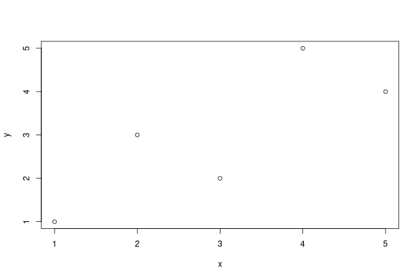
y <- c(1,3,2,5,4)
x <- c(1,2,3,4,5)
plot(x,y)
demo <- glm(y~x,family='poisson')
fit <- fitted(demo)
dev <- 0
for (i in 1:5) {
    dev <- dev + (y[i] * log(y[i]/fit[i]) - (y[i]-fit[i]))
}
dev <- dev * 2
dev
1.42328
To get the null deviance we simply apply the mean of \(y\) as the fitted value
for each case.
null.dev <- 0
for (i in 1:5) {
    null.dev <- null.dev + (y[i] * log(y[i]/mean(y)) - (y[i]-mean(y)))
}
null.dev <- null.dev * 2
null.dev
[1] 3.590628
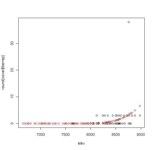
bere6.glm <- glm(round(cover$berrep) ~ elev + I(elev^2),family='poisson')
summary(bere6.glm)
This was not too successful. The problem is that the values are highly skewed,
with mostly zeros, and a single very high value.
Call:
glm(formula = round(cover$berrep) ~ elev + I(elev^2), family = "poisson")

Deviance Residuals:
      Min         1Q     Median         3Q        Max
-2.773616  -0.548849  -0.119568  -0.006365  10.734024

Coefficients:
              Estimate Std. Error z value Pr(>|z|)
(Intercept) -1.948e+02  1.063e+02  -1.833   0.0668 .
elev         4.124e-02  2.484e-02   1.660   0.0969 .
I(elev^2)   -2.153e-06  1.451e-06  -1.484   0.1379
---
Signif. codes:  0 '***' 0.001 '**' 0.01 '*' 0.05 '.' 0.1 ' ' 1

(Dispersion parameter for poisson family taken to be 1)

    Null deviance: 504.37  on 159  degrees of freedom
Residual deviance: 266.05  on 157  degrees of freedom
AIC: 337.36

Number of Fisher Scoring iterations: 7
plot(elev,round(cover$berrep))
points(elev,fitted(bere6.glm),col=2)
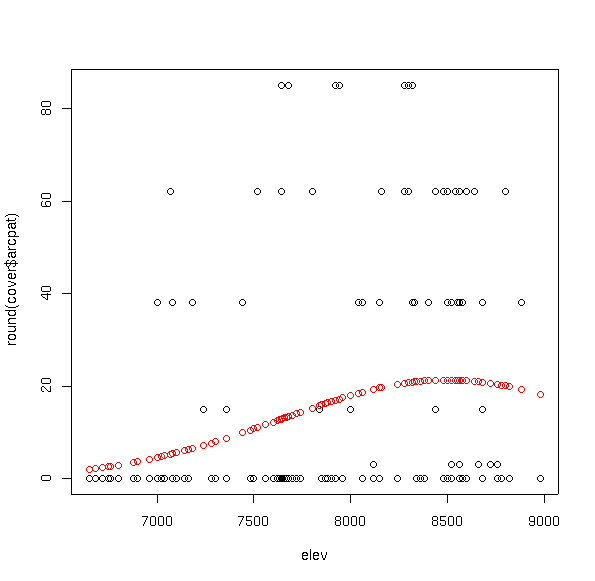
arpa.glm <- glm(round(cover$arcpat) ~ elev + I(elev^2),family='poisson')
summary(arpa.glm)
Here we were much more successful, as you can see.
Call:
glm(formula = round(cover$arcpat) ~ elev + I(elev^2), family = "poisson")

Deviance Residuals:
   Min      1Q  Median      3Q     Max
-6.529  -5.724  -4.632   2.722  13.888

Coefficients:
              Estimate Std. Error z value Pr(>|z|)
(Intercept) -4.657e+01  4.590e+00 -10.147   <2e-16 ***
elev         1.168e-02  1.152e-03  10.136   <2e-16 ***
I(elev^2)   -6.871e-07  7.214e-08  -9.526   <2e-16 ***
---
Signif. codes:  0 '***' 0.001 '**' 0.01 '*' 0.05 '.' 0.1 ' ' 1

(Dispersion parameter for poisson family taken to be 1)

    Null deviance: 6018.6  on 159  degrees of freedom
Residual deviance: 5479.2  on 157  degrees of freedom
AIC: 5774.6

Number of Fisher Scoring iterations: 7
plot(elev,round(cover$arcpat))
points(elev,fitted(arpa.glm),col=2)
References
Functions Used In This Lab
thresh <- function(obs,fitted)
{
    N <- length(obs)
    Z <- 1:N

    obs <- obs[rev(order(fitted))]
    fitted <- fitted[rev(order(fitted))]
    P <- sum(fitted)

    a <- cumsum(fitted)
    b <- cumsum(1-fitted)
    c <- P - a
    d <- N - (a+b+c)

    ppp <- a/Z
    sens <- a/(a+c)
    spec <- d/(b+d)
    kappa <- ((a+d)/N - ((a+b)*(a+c) + (c+d)*(d+b))/N^2)/
              (1-((a+b)*(a+c) + (c+d)*(d+b))/N^2)

    tss <- sens + spec - 1
    acc <- (a+d)/N
    max.tss <- which.max(tss)
    max.kap <- which.max(kappa)
    max.acc <- which.max(acc)

    vecs <- data.frame(obs,fitted,a,b,c,d,sens,spec,tss,kappa,acc=acc)
    tholds <- data.frame(c(max.kap,max.tss,max.acc),
                         c(fitted[max.kap],fitted[max.tss],fitted[max.acc]),
                         c(kappa[max.kap],tss[max.tss],acc[max.acc]),
                         c(a[max.kap],a[max.tss],a[max.acc]),
                         c(b[max.kap],b[max.tss],b[max.acc]),
                         c(c[max.kap],c[max.tss],c[max.acc]),
                         c(d[max.kap],d[max.tss],d[max.acc]))

    plot(Z,sens,col=2,ylim=c(0,1),type='l',lwd=3,
          xlab='Rank',ylab='Index')
    points(Z,spec,col=4,type='l',lwd=3)
    points(Z,tss,col=3,type='l',lwd=3)
    points(Z,acc,col=5,type='l',lwd=3)
    points(Z,kappa,col='grey',type='l',lwd=3)

    abline(v=max.tss,col=3,lty=2)
    abline(v=max.kap,col='grey',lty=2)
    abline(v=max.acc,col=5)
    abline(v=sum(obs),lty=3)
    text(N,0.9,'Sn',col=2,adj=1)
    text(N,0.8,'Sp',col=4,adj=1)
    text(N,0.7,'TSS',col=3,adj=1)
    text(N,0.6,'ACC',col=5,adj=1)
    text(N,0.5,'Kappa',col='grey',adj=1)

    names(tholds) <- c('rank','pval','value','a','b','c','d')
    row.names(tholds) <- c('kappa','TSS','ACC')
    print(tholds)
    out <- list(vecs=vecs,tholds=tholds)
    invisible(out)
}