In this lab we want to know the degree to which plot membership in a cluster is predictable from environmental variables not used in the classification. There are several reasons we might want to pursue this effort. Similar to our efforts with fitting surfaces on ordinations, one important reason is to determine the relationship between environmental variability and vegetation composition. Here we approaching the question with a less continuous variability. More important than interpretation, however, is the potential for prediction. That is, given environmental variables, can we predict vegetation composition? Back in Labs 4 and 5 we tried to predict the presence/absence or abundance of single species, but here we're predicting total community composition within classes or types. Specifically, rather than try to predict a single value (presence or abundance), we're trying choose among a set of possible alternatives. Every plot must be assigned to a type.
Among the variety of techniques available to us (e.g. linear discriminant analysis (LDA) and quadratic discriminant analysis (QDA)) in this lab we will emphasize tree-based classifiers. Tree classifiers are often called CART (for Classification And Regression Trees), but CART is actually a specific (copyrighted and trade-marked) example of such approaches. In R the tree classifier is called tree() To get started, we need to load somae packages.
library(optpart)
library(tree)
data(brycesite)
data(bryceveg)
attach(brycesite)
hcl1 <- hclust(dis.bc,method="complete")
plot(hcl1)
As we've seen before, using the "complete" method leads to discrete clusters at 1.0 dissimilarity. I'll slice the tree at 0.99 to generate clusters.
hcl1.99 <- cutree(hcl1,h=0.99)
table(hcl1.99)
 1  2  3  4  5  6  7  8
38 46 17  2 14 32  7  4
opt5 <- optpart(5,dis.bc)
table(opt5$clustering)
 1  2  3  4  5
38 92 14 12  4
plot(tree1)
text(tree1)
The tree is shown with the root at the top, and each sequential split along each branch is labeled with the respective criterion for splitting. Values that are true go left; values that are false go right. The height of the vertical bar above each split reflects the decrease in deviance associated with that split. To see the output, just type it's name.
Once we split, we simply proceed with the same objective independently for each branch on the remaining data. For example, on branch 2, where we now have 83 plots, the next split is
  4) elev < 7580 34  87.550 3 ( 0.00000 0.14706 0.38235 ... 0.00000 0.05882)
  5) elev > 7580 49  95.200 6 ( 0.00000 0.20408 0.00000 ... 0.14286 0.00000)
To see a simple summary of the results, enter
Classification tree:
tree(formula = factor(hcl1.99) ~ elev + av + slope + depth +
    pos)
Variables actually used in tree construction:
[1] "elev"  "pos"   "slope" "av"
Number of terminal nodes:  13
Residual mean deviance:  0.7428 = 98.05 / 132
Misclassification error rate: 0.131 = 19 / 145
If there are eight types, why are there 13 terminal nodes? For some types there is more than one route to a terminal node. For example, nodes 22, 23, and 42 all predict cluster 6. Nodes 22 and 23 are a single split, and yet both predict cluster 6. Why is that? Node 22 predicts type 6 perfectly (p=1.0, dev.=0) while node 23 is less clean (p=0.60, dev.=6.73). Splitting node 11 into 22 and 23 achieved a reduction in deviance of 14.560 - (6.730+0.000) = 7.83 with a single split, even though both branches predicted the same type. Less obvious at first glance, is that some types or clusters were never predicted at all. None of the terminal nodes predicts types 4 or 8. There are simply too few plots in those types to predict accurately, and they fall below the minimum splitting rule of at least 5 plots/type.
The misclassification error is 19 out of 145, or 0.131 or 13%. That's good enough for practical purposes probably. We could calculate a probability of getting 126/145 correct given our initial distribution, but it's bound to be very significant. Of more interest perhaps is which types were confused with which other types. We can view this in a table called a "confusion matrix." In package optpart there is a confusion matrix function called confus(). It requires at least two arguments: a clustering, and a tree model. In this case we need to be careful about the missing values.
confus(hcl1.99[!is.na(depth)],tree1)
$confus
     [,1] [,2] [,3] [,4] [,5] [,6] [,7] [,8]
[1,]   36    1    0    0    0    0    0    0
[2,]    5   30    1    0    0    3    1    0
[3,]    0    2   10    0    1    0    0    0
[4,]    0    1    0    0    0    1    0    0
[5,]    0    0    0    0   13    0    0    0
[6,]    0    1    0    0    0   30    0    0
[7,]    0    0    0    0    0    0    7    0
[8,]    0    1    1    0    0    0    0    0

$correct
[1] 126

$percent
[1] 0.8689655

$kappa
[1] 0.8342359
In addition, confus() provides the number of correct predictions, the percent correct predictions, and the \(\kappa\) statistic.
As for our experience modeling species with trees, the trees are over-fit and need to be pruned by cross-validation.
plot(cv.tree(tree1),type='b',ylim=c(200,600))
for (i in 1:10) {
     x <- cv.tree(tree1)
     points(x$size,x$dev,type='b')
}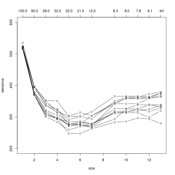
tree1.5 <- prune.tree(tre1,best=5)
tree1.5
summary(tree1.5)
tree1.5
node), split, n, deviance, yval, (yprob)
      * denotes terminal node

 1) root 145 501.900 2 ( 0.25517 0.27586  ... 0.01379 0.08966 0.21379 0.04828 0.01379 )
   2) elev < 7980 83 273.200 6 ( 0.00000 0.18072  ... 0.15663 0.37349 0.08434 0.02410 )
     4) elev < 7580 34  87.550 3 ( 0.00000 0.14706  ...0.38235 0.00000 0.00000 0.05882 )
       8) elev < 6980 14   7.205 5 ( 0.00000 0.00000  ...0.00000 0.00000 0.00000 ) *
       9) elev > 6980 20  41.320 3 ( 0.00000 0.25000  ... 0.00000 0.00000 0.10000 ) *
     5) elev > 7580 49  95.200 6 ( 0.00000 0.20408  ... 0.00000 0.63265 0.14286 0.00000 )
      10) slope < 2.5 20  48.230 2 ( 0.00000 0.40000  ... 0.00000 0.20000 0.35000 0.00000 ) *
      11) slope > 2.5 29  14.560 6 ( 0.00000 0.06897  ... 0.00000 0.93103 0.00000 0.00000 ) *
   3) elev > 7980 62  83.610 1 ( 0.59677 0.40323  ... 00000 0.00000 0.00000 0.00000 0.00000 ) *
Classification tree:
snip.tree(tree = tree1, nodes = c(11L, 9L, 10L, 3L))
Variables actually used in tree construction:
[1] "elev"  "slope"
Number of terminal nodes:  5
Residual mean deviance:  1.392 = 194.9 / 140
Misclassification error rate: 0.331 = 48 / 145
confus(hcl1.99[!is.na(depth)],tree1.5)
 $confus
     [,1] [,2] [,3] [,4] [,5] [,6] [,7] [,8]
[1,]   37    0    0    0    0    0    0    0
[2,]   25    8    5    0    0    2    0    0
[3,]    0    0   12    0    1    0    0    0
[4,]    0    1    1    0    0    0    0    0
[5,]    0    0    0    0   13    0    0    0
[6,]    0    4    0    0    0   27    0    0
[7,]    0    7    0    0    0    0    0    0
[8,]    0    0    2    0    0    0    0    0

$correct
[1] 97

$percent
[1] 0.6689655

$kappa
[1] 0.5804702
How about our other classification using optpart?
tree2 <- tree(factor(opt5$clustering) ~ elev + av + slope + depth + pos)
plot(tree2)
text(tree2)
node), split, n, deviance, yval, (yprob)
      * denotes terminal node

 1) root 145 326.600 2 ( 0.25517 0.57931 0.08966 0.04828 0.02759 )
   2) elev < 7980 83 225.300 1 ( 0.44578 0.26506 0.15663 ... 0.04819 )
     4) elev < 7580 34  71.970 2 ( 0.00000 0.41176 0.38235 ... 0.00000 )
       8) elev < 6980 14   7.205 3 ( 0.00000 0.07143 0.92857 ... 0.00000 ) *
       9) elev > 6980 20  25.900 2 ( 0.00000 0.65000 0.00000 ... 0.00000 )
        18) pos: bottom,low_slope,mid_slope,ridge 12   6.884 2 ( 0.00000
                                    0.91667 0.00000 0.08333 0.00000 ) *
        19) pos: up_slope 8   8.997 4 ( 0.00000 0.25000 ... 0.00000 ) *
     5) elev > 7580 49  69.830 1 ( 0.75510 0.16327 0.00000  ... 0.08163 )
      10) slope < 2.5 20  42.200 1 ( 0.40000 0.40000 0.00000 ... 0.20000 )
        20) elev < 7845 10  12.220 2 ( 0.30000 0.70000 ... 0.00000 ) *
        21) elev > 7845 10  18.870 1 ( 0.50000 0.10000  ... 0.40000 )
          42) av < 0.58 5   5.004 1 ( 0.80000 0.00000  ... 0.20000 ) *
          43) av > 0.58 5   9.503 5 ( 0.20000 0.20000 ... 0.60000 ) *
      11) slope > 2.5 29   0.000 1 ( 1.00000 0.00000  ... 0.00000 ) *
   3) elev > 7980 62   0.000 2 ( 0.00000 1.00000  ... 0.00000 0.00000 ) *
Classification tree:
tree(formula = factor(opt5$clustering) ~ elev + av + slope + depth +
    pos)
Variables actually used in tree construction:
[1] "elev"  "pos"   "slope" "av"
Number of terminal nodes:  8
Residual mean deviance:  0.3636 = 49.81 / 137
Misclassification error rate: 0.06897 = 10 / 145
plot(cv.tree(tree2),type='b',ylim=c(100,400))
for (i in 1:10) {
x <- cv.tree(tree2)
points(x$size,x$dev,type='b')
}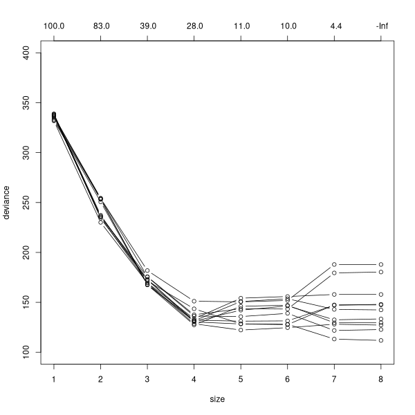 Assuming (somewhat generously) that 6 is the best number:
tree2.6 <- prune.tree(tree2,best=6)
confus(opt5$clustering[!is.na(depth)],tree2.6)
$confus
     [,1] [,2] [,3] [,4] [,5]
[1,]   82    1    0    1    0
[2,]    3   34    0    0    0
[3,]    7    0    0    0    0
[4,]    0    0    0   13    0
[5,]    0    4    0    0    0

$correct
[1] 129

$percent
[1] 0.8896552

$kappa
[1] 0.8012337
 confus <- function (clustering, model, diss = NULL)
{
    clustering <- clustify(clustering)
    if (inherits(model, "tree")) {
        fitted <- predict(model)
    }
    else if (inherits(model, "randomForestest")) {
        fitted <- predict(model, type = "prob")
    }
    else if (inherits(model, "matrix")) {
        fitted <- model
    }
    numplt <- length(clustering)
    numclu <- length(levels(clustering))
    pred <- apply(fitted, 1, which.max)
    res <- matrix(0, nrow = numclu, ncol = numclu)
    for (i in 1:numplt) {
        res[clustering[i], pred[i]] <- res[clustering[i], pred[i]] +
            1
    }
    if (!is.null(diss)) {
        part <- partana(clustering, diss)
        shunt <- diag(part$ctc)
        shunt[shunt == 0] <- 1
        tmp <- part$ctc/shunt
        fuzerr <- 1 - matrix(pmin(1, tmp), ncol = ncol(tmp))
        diag(fuzerr) <- 1
        fuzres <- res
        for (i in 1:ncol(res)) {
            for (j in 1:ncol(res)) {
                if (i != j) {
                  fuzres[i, j] <- res[i, j] * fuzerr[i, j]
                  fuzres[i, i] <- fuzres[i, i] + res[i, j] *
                    (1 - fuzerr[i, j])
                }
            }
        }
        res <- fuzres
    }
    correct <- sum(diag(res))
    percent <- correct/numplt
    rowsum <- apply(res, 1, sum)
    colsum <- apply(res, 2, sum)
    summar <- sum(rowsum * colsum)
    kappa <- ((numplt * correct) - summar)/(numplt^2 - summar)
    out <- list(confus = res, correct = correct, percent = percent,
        kappa = kappa)
    out
}
isolate <- function (mod,thresh=0.1)
{
    if (inherits(mod,'randomForest')) {
        tab <- mod$confus
    } else if (inherits(mod,'tree')) {
        tab <- confus(mod$y,mod)$confus
        rownames(tab) <- as.character(1:nrow(tab))
        colnames(tab) <- as.character(1:ncol(tab))
    } else {
        stop("Model type not recognized")
    }
    size <- nrow(tab)

    for (i in 1:(size-1)) {
        for (j in (i+1):size) {
            num <- tab[i,j] + tab[j,i]
            denom <- tab[i,i] + tab[j,j] +tab[i,j] + tab[j,i]
            if (denom > 0) {
                if (((tab[i,j] + tab[j,i]) / (tab[i,i] + tab[j,j] +tab[i,j] + tab[j,i]))
                          > thresh) {
                    a <- c(tab[i,i],tab[j,i])
                    b <- c(tab[i,j],tab[j,j])
                    out <- data.frame(a,b)
                    names(out) <- colnames(tab)[c(i,j)]
                    row.names(out) <- colnames(tab)[c(i,j)]
                    cat('\n')
                    print(out)
                }
            }
        }
    }
}