Lab 13 — Cluster Analysis
Cluster analysis is a multivariate analysis that attempts to form groups
or "clusters" of objects (sample plots in our case) that are "similar"
to each other but which differ among clusters.
The exact definition of "similar" is variable among algorithms,
but has a generic basis. The methods of forming clusters also vary, but
follow a few general blueprints.
Similarity, Dissimilarity and Distance
Similarity is a characterization of the ratio of
the number of attributes two objects share in common compared to the total list
of attributes between them. Objects which have everything in common are
identical, and have a similarity of 1.0. Objects which have nothing in common
have a similarity of 0.0. As we have discussed previously (see Lab 8), there is a large
number of similarity indices proposed and employed, but the concepts are
common to all.
Dissimilarity is the complement of similarity, and is a characterization of the
number of attributes two objects have uniquely compared to the total list
of attributes between them. In general, dissimilarity can be calculated as
1 - similarity.
Distance is a geometric conception of the proximity of objects in a high
dimensional space defined by measurements on the attributes. We've covered
distance in detail under "ordination by PCO", and I refer you to that discussion
for more details. Remember that R calculates distances with the dist
function, and uses "euclidean", "manhattan", or "binary" as the "metric." The
vegan package provides vegdist(), and labdsv provides dsvdis
which together provide a large number of possible indices and metrics.
Similar to the way in which these indices and metrics influenced ordination
results, they similarly influence cluster analyses.
In practice, distances and dissimilarities are sometimes
used interchangeably. They have quite distinct properties, however.
Dissimilarities are bounded [0,1]; once plots have no species in common
they can be no more dissimilar. Distances are unbounded on the upper end;
plots which have no species in common have distances that depend on the number
and abundance of species in the plots, and is thus variable.
Cluster Algorithms
Cluster algorithms are classified by two characteristics: (1) hierarchical
vs fixed-cluster, and (2) if hierarchical, agglomerative vs divisive. We will
explore agglomerative hierarchical clusters first, followed by fixed cluster
and fuzzy fixed-cluster methods next.
In agglomerative hierarchical cluster analysis, sample plots all start out
as individuals, and the two plots most similar (or least dissimilar) are
fused to form the first cluster. Subsequently, plots are continually fused
one-by-one in order of highest similarity (or equivalently lowest dissimilarity) to
the plot or cluster to which they are most similar. The hierarchy is determined
by the cluster at a height characterized by the similarity at which the plots
fused to form the cluster. Eventually, all plots are contained in the final
cluster at similarity 0.0
Agglomerative cluster algorithms differ in the calculation of similarity when
more than one plot is involved; i.e. when a plot is considered for merger
with a cluster containing more than one plot. Of all the algorithms invented,
we will limit our consideration to those available in R, which are also
those most commonly used. In R there are multiple methods:
- single --- nearest neighbor
- complete --- furthest neighbor or compact
- ward --- Ward's minimum variance method
- mcquitty --- McQuitty's method
- average --- average similarity
- median --- median (as opposed to average) similarity
- centroid --- geometric centroid
- flexible --- flexible Beta
In the "connected" or "single" linkage, the similarity of a plot to a cluster is
determined by the maximum similarity of the plot to any of the plots in the
cluster. The name "single linkage" comes because the plot only needs to be
similar to a single member of the cluster to join. Single linkage clusters
can be long and branched in high-dimensional space, and are subject to a
phenomenon called "chaining", where a single plot is continually added to the
tail of the biggest cluster. On the other hand, single linkage clusters are
topologically "clean."
In the average linkage, the similarity of a plot to a cluster is defined by
the mean similarity of the plot to all the members of the cluster. In contrast to
single linkage, a plot needs to be relatively similar to all the members of the
cluster to join, rather than just one. Average linkage clusters tend to be
relatively round or ellipsoid. Median or centroid approaches tend to give
similar results.
In the "complete" linkage, or "compact" algorithm, the similarity of a plot
to a cluster is calculated as the minimum similarity of the plot to any
member of the cluster. Similar to the single linkage algorithm, the probability
of a plot joining a cluster is determined by a single other member of a cluster,
but now it is the least similar, not the most similar. Complete linkage clusters
tend to be very tight and spherical, thus the alternative name "compact."
Hierarchical Cluster Analysis in R
To perform cluster analysis you will want to load two packages: cluster
and optpart. cluster is a package originally contributed by
Kauffmann, but now maintained by Maechler et al. (2019). This package includes
many of the famous algorithms ffrom Kaufman and Rousseeuw in their text
"Finding Groups in Data." optpart is by Roberts and includes the
algorithms featured in Roberts (2015).
In R, we typically use the hclust() function to perform hierarchical
cluster analysis. hclust() will calculate a cluster analysis from either
a similarity or dissimilarity matrix, but plots better when working from a
dissimilarity matrix. We can use any dissimilarity object from
dist(), vegdist(), or dsvdis().
Give the hclust() function the dissimilarity object as the first
argument, and the method or metric as the second explicit argument. E.g.
hcl.avg <- hclust(demodist,"average")
To see the cluster analysis, simply use the plot().
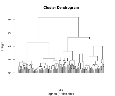
plot(hcl.avg)
The hierarchical cluster analysis is drawn as a "dendrogram", where each fusion
of plots into a cluster is shown as a horizontal line, and the plots are
labeled at the bottom of the graph (although often illegibly in dense
graphs).
I prefer a more traditional representation where the lines come all the way
down. You can get that with
plot(hcl.avg,hang=-1,labels=NA)

The cluster analysis can be "sliced" horizontally to produce unique clusters
either by specifying a similarity or the number of clusters desired. For
example, to get 5 clusters, use
avg.5 <- slice(hcl.avg,k=5)
Then, to label the dendrogram with the group IDs, use
plot(hcl.avg, labels = as.character(hcl.5$clustering))
Given the clusters, you can use the cluster IDs (in our case avg.5) as
you would any categorical variable. For example,
table(berrep,avg.5$clustering)
      1  2  3  4 5
   0 39 21 14 17 1
 0.5  0 47  0  0 0
   3  0 20  0  0 0
37.5  0  1  0  0 0
You can also perform environmental analyses of the clusters using the
various plotting techniques we have developed. For example, to look
at the distribution of plot elevations within clusters, we can do a
boxplot as follows (assuming that the site data are already attached):
boxplot(elev~avg.5t$clustering)
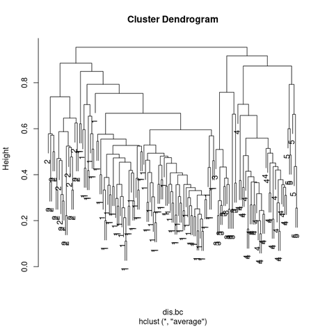
As another example, I'll use complete on the Bray/Curtis
dissimilarity calculated in a previous lab
and then follow with const()
hcl.comp <- hclust(dis.bc,"complete")
Notice how in the "complete" dendrogram clusters tend to hang from the 1.0
dissimilarity line. This is because the similarity of each cluster to the
others is defined by the least similar pairs among the two, which is often
complete dissimilarity. If we cut this at 0.99, we get 8 clusters that are
distinct.
hcl.comp.99 <- cutree(hcl.comp,h=0.99)
R version 4 broke some code in optpart, so to use const(),
importance() or concov() you need to paste the functions in from
down below. const() shows the constancy (fraction of sample units
where a species is present) by type. The argument min= specifies the
minimum constancy for a species' constancy to show up in the table, allowing you
to focus on common or dominant species.
const(bryceveg,hcl.comp.99,min=0.2)
          1    2    3    4    5    6    7    8
ameuta 0.34 0.21  .    .    .    .    .    .
arcpat 0.71 0.89 0.23  0.5  .    .    .   0.25
arttri  .    .    .    .   0.85  .    .   0.25
atrcan  .    .    .    .   0.92  .    .    .
ceamar 0.52 0.84  .    .    .    .    .    .
cermon  .   0.28 0.94  .    .    .    .   1.00
  .     .    .    .    .    .    .    .    .
  .     .    .    .    .    .    .    .    .
  .     .    .    .    .    .    .    .    .
senmul 0.60 0.47  .    .    .   0.78 0.28  .
sphcoc  .    .    .    .   0.64  .    .    .
swerad 0.26 0.32  .    .    .    .    .    .
taroff  .    .    .    .    .    .   0.42  .
towmin  .    .    .    1.0  .    .    .    .
tradub  .    .    .    .   0.21 0.21  .    .
Flexible-Beta
In recent years many ecologists have expressed a preference for a hierarchical
clustering algorithm call "flexible Beta" developed by Australian ecologists
Lance and Williams (1966). Lance and Williams determined that since all
hierarchical agglomerative algorithms operate similarly, but differ in the
calculation of multi-member dissimilarity, that it was possible to generalize
the algorithms to a single algorithm with four parameters, alpha_1, alpha_2,
beta, and gamma. Legendre and Legendre (1998) present a table (Table 8.8) that
gives the L&W parameters to recreate many of the classical algorithms. Of more
interest here is a special case where alpha_1 = alpha_2 = 0.625, beta = -0.25,
and gamma = 0. Observe that not only are alpha_1 and alpha_2 equal, but that it
is also the case that beta = 1 - (alpha_1 + alpha_2). This set of parameters
gives a good intermediate result. To use flexible-beta in R you must load the
package "cluster." This package contains several other functions we will want.
Package "cluster" is loaded automatically by package "optpart", but if you have
not loaded either yet
library(cluster)
The function we want to use is called agnes() (an abbreviation for
agglomerative nesting). To perform a flexible-beta using agnes(), the
call is a little more complicated than we have seen for other clustering
algorithms). We need to specify alpha_1, alpha_2, beta, and beta in the call,
using the par.method argument.
demoflex <- agnes(dis.bc,method='flexible',par.method=c(0.625,0.625,-0.25))
The defaults, however, are that alpha_1 = alpha_2, beta = 1 - (alpha_1 + alpha_2),
and gamma = 0. So we can simply specify alpha_1 and get the desired results.
demoflex <- agnes(dis.bc,method='flexible',par.method=0.625)
Alternatively, package optpart has a wrapper fopr agnes() to get
flexible-\(\beta\) the way ecologists usually refer to it.
hcl.fb <- flexbeta(dis.bc,beta=-0.25)
plot(hcl.fb,hang=-1,labels=FALSE)
Cluster Utilities and Cluster Validity Indices
Hierarchical clustering can be challenging to manage. You not only have to
decide: (1) what distance/dissimilarity to use, (2) which algorithm to use, but
also (3) where to cut the dendrogram to produce clusters. Finally, when you are
done, you need to evaluate the goodness-of-clustering. In combination, packages
:cluster" and "optpart" can be very helpful here. First let's talk about
goodness-of-clustering tests.
Goodness-of-Clustering
Aho et al. (2008) characterize goodness-of-clustering test as falling into two
groups: internal and external. Internal tests are based on the
distance/dissimilarity matrices that were used to create the partition, whereas
external tests are based on data outside the construction of the dendrogram or
the partition, such as environmental variables. In this section I will
emphasize internal evaluators.
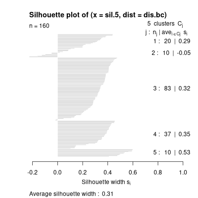
P.J. Rousseeuw (1987) developed a diagnostic called "silhouette plots" that show
the goodness-of-fit of each cluster member to the cluster and the hoomogeneity
of each cluster. The graphic and statistic is based "silhouette width."
\[ s_i = (b_i - a_i) / \max(a_i,b_i)\]
where \(s_i\) is the silhouette width of sample unit \(i\), \(a_i\) is the mean
dissimilatrity of sample unit \(i\) to its assigned cluster, and
\(b_i\) is the mean
dissimilarity of sample unit \(i\) to the cluster it is least dissimilar to
(nearest neighbor cluster) aside from the one it is assigned to.
\[s_i \sim [-1,1]\]
Sample units that are less dissimilar to their assigned cluster than to their
nearest neighbor have positive silhouette widths, and sample units that are less
dissimilar to their nearest neighbor then to their assigned cluster have
negative silhouette widths, and can be considered "mis-fits."
To plot a silhouette plot yu need (12) a cluster solution, and (2) a
distance/dissimilarity matrix.
plot(silhouette(hcl.5,dis.bc))
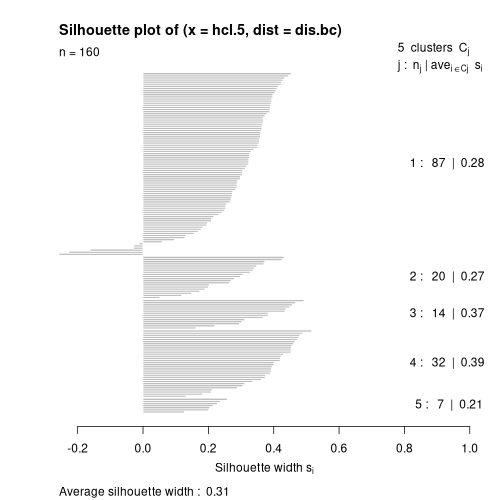 What you see is (1) cluster 1 has 87 members with a mean width of 0.28, cluster
2 has 20 members with a mean width of 0.27, etc., and that the overall mean
cluster width is 0.31 (which is pretty good). You also see that cluster 1 has
several negative silhouette widths (or "reversals") and that maybe some plots
are mis-assigned. You can compare results of other cluster solutions by
comparing (1) the mean silhouette width, and (2) the number of reversals.
Roberts (see Aho et al. 2008) proposed "partition analysis" as a way to
evaluate partitions. It calculates (1) the mean similarity of each element to
each cluster, (2) the mean similarity of each cluster to itself and every other
cluster, and (3) importantly, the ratio of within-cluster similarity to between
cluster similarity.
What you see is (1) cluster 1 has 87 members with a mean width of 0.28, cluster
2 has 20 members with a mean width of 0.27, etc., and that the overall mean
cluster width is 0.31 (which is pretty good). You also see that cluster 1 has
several negative silhouette widths (or "reversals") and that maybe some plots
are mis-assigned. You can compare results of other cluster solutions by
comparing (1) the mean silhouette width, and (2) the number of reversals.
Roberts (see Aho et al. 2008) proposed "partition analysis" as a way to
evaluate partitions. It calculates (1) the mean similarity of each element to
each cluster, (2) the mean similarity of each cluster to itself and every other
cluster, and (3) importantly, the ratio of within-cluster similarity to between
cluster similarity.
summary(partana(avg.5,dis.bc))
Number of clusters =  5

 1  2  3  4  5
87 20 14 32  7

           [,1]        [,2]       [,3]       [,4]        [,5]
[1,] 0.37692189 0.115167420 0.01784878 0.05814787 0.051498315
[2,] 0.11516742 0.364767129 0.04080794 0.04945133 0.009980879
[3,] 0.01784878 0.040807939 0.42732677 0.09399166 0.033791447
[4,] 0.05814787 0.049451332 0.09399166 0.48048127 0.127317729
[5,] 0.05149832 0.009980879 0.03379145 0.12731773 0.318411602

Ratio of Within-cluster similarity/Among-cluster similarity =  5.954
plot(partana(avg.5,dis.bc))
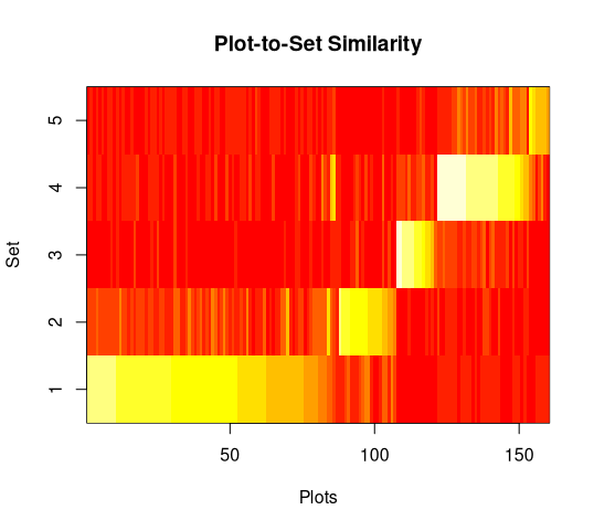 The first panel shows the similarity of each sample unit to each cluster, with
high similarities in white or yellow and low similarities in red. Sample units
are sorted in order of their similarity to their assigned cluster. In this
example yu can see that a few sample units assigned to cluster 1 are more
similar to cluster 4 than they are to cluster 1, but that over all the results
are pretty good (bright yellow on the diagonal and red off the diagonal).
The first panel shows the similarity of each sample unit to each cluster, with
high similarities in white or yellow and low similarities in red. Sample units
are sorted in order of their similarity to their assigned cluster. In this
example yu can see that a few sample units assigned to cluster 1 are more
similar to cluster 4 than they are to cluster 1, but that over all the results
are pretty good (bright yellow on the diagonal and red off the diagonal).
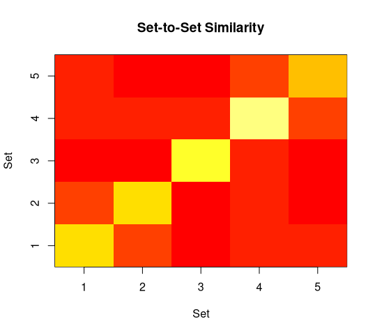 The second panel ignores the individual sample units and just displays cluster
means. You can see a slight similarity of cluster 1 to cluster 2 (faint orange
off the diagonal), that cluster 4 and 5 are slightly similar (same criterion),
and that cluster 4 has the highest homogeneity (brightest yellow) while cluster
is not so good.
The second panel ignores the individual sample units and just displays cluster
means. You can see a slight similarity of cluster 1 to cluster 2 (faint orange
off the diagonal), that cluster 4 and 5 are slightly similar (same criterion),
and that cluster 4 has the highest homogeneity (brightest yellow) while cluster
is not so good.
Selecting the Number of Clusters
Now that you have seen the silhouette width and partana ratio
goodness-of-clustering analyses, you have a basis to compare different
clustering results, including the best number of clusters. To facilitate that,
the optpart package ahs the stride() command.
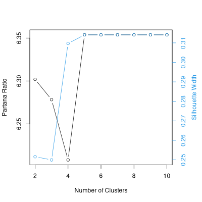
stride() slices a dendrogram at as many points as desired, using an R
sequence to specify. For example
avg.3.10 <- stride(3:10,hcl.avg)
The resulting stride object can then be analyzed by silhouette width or
partana ratio.
silhouette(avg.3.10,dis.bc)
  clusters sil_width
1        3 0.2754676
2        4 0.2971435
3        5 0.3066199
4        6 0.2906381
5        7 0.2753434
6        8 0.2747093
7        9 0.2778687
8       10 0.2438136
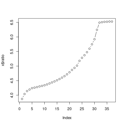
partana(avg.3.10,dis.bc)
  clusters    ratio
1        3 6.246947
2        4 5.924215
3        5 5.953795
4        6 5.936849
5        7 5.599706
6        8 5.596239
7        9 5.569672
8       10 5.519177
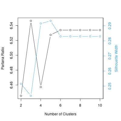
plot(avg.3.10,dis.bc)
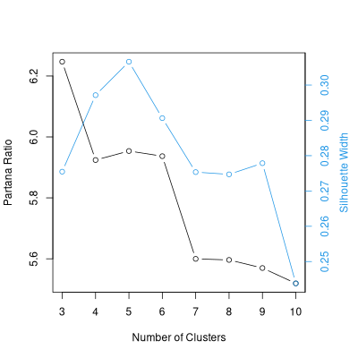 Given this results, 3 or 5 cluster looks good, and there is no reason to prefer
4 or 6 over those two, and certainly higher numbers of clusters give poorer
results.
Given this results, 3 or 5 cluster looks good, and there is no reason to prefer
4 or 6 over those two, and certainly higher numbers of clusters give poorer
results.
Fixed-cluster Algorithms or Partitions
In contrast to hierarchical methods,
in fixed-cluster algorithms (e.g. C-means, K-means or K-medoids), the
number of clusters is specified a priori by the analyst,
and the clusters are formed from either an initial guess at the
cluster centers, or from random initial conditions. The clusters
are not hierarchical, but rather form a direct partition of the data.
The "goodness-of-fit" criterion (also called "stress")
is generally some measure of
within-cluster homogeneity versus among-cluster
heterogeneity, often measured by the distance of each plot to the
center of the cluster to which it belongs, compared to the average
distance to other clusters.
In practice, you often don't know the best number of clusters
a priori, and the approach adopted is to cluster at a range
of values, comparing the stress values to find the best partition.
Often, clustering with the same number of clusters but a different
initial guess will lead to a different final partition, so
replicates at each level are often required.
The original function for fixed-cluster analysis was called "K-means" and
operated in a Euclidean space. Kaufman and Rousseeuw (1990) created a function
called "Partitioning Around Medoids" (PAM) which operates with any of a broad
range of dissimilarities/distance.
To perform fixed-cluster analysis in R we'll use the pam()
function from the cluster library.
pam uses a distance matrix output from any of our distance functions,
or a raw vegetation matrix (invoking dist() on the fly).
I've had better luck explicitly creating a distance matrix first, and
then submitting it to pam.
pam.5 <- pam(dis.bc,k=5)
attributes(pam.5)
$names:
[1] "medoids"    "id.med"     "clustering" "objective"  "isolation"
[6] "clusinfo"   "silinfo"    "diss"       "call"

$class:
[1] "pam"       "partition"
pam.5$medoids
[1] "bcnp_64" "bcnp__7" "bcnp103" "bcnp159" "bcnp_88"
The cluster membership for each plot is given by
pam.5$clustering
bcnp__1 bcnp__2 bcnp__3 bcnp__4 bcnp__5 bcnp__6 bcnp__7 bcnp__8
      1       1       1       1       2       1       2       2
bcnp__9 bcnp_10 bcnp_11 bcnp_12 bcnp_13 bcnp_14 bcnp_15 bcnp_16
      1       2       2       2       1       2       2       1
      .       .       .       .       .       .       .       .
      .       .       .       .       .       .       .       .
      .       .       .       .       .       .       .       .
bcnp145 bcnp146 bcnp147 bcnp148 bcnp149 bcnp150 bcnp151 bcnp152
      4       4       4       4       4       4       4       4
bcnp153 bcnp154 bcnp155 bcnp156 bcnp157 bcnp158 bcnp159 bcnp160
      4       4       4       4       4       4       4       4
plot(pam.5)
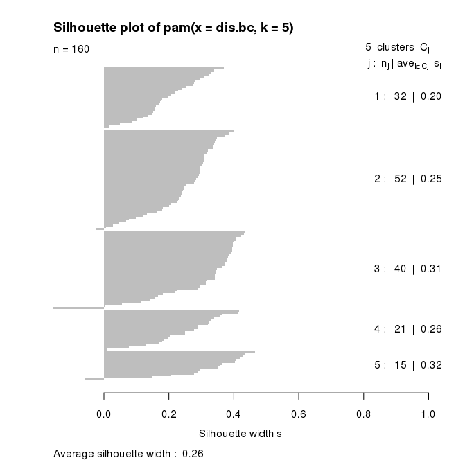
for pam(), the default plot is a silhouette plot.
- the number of plots per cluster = number of horizontal lines, also given in
the right hand column,
- the means similarity of each plot to its own cluster
minus the mean
similarity to the next most similar cluster (given by the length of the lines)
with the mean in the right hand column, and
-
the average silhouette width
Plots which fit well within their cluster have a large positive Silhouette
width; those which fit poorly have a small positive or even a negative
Silhouette.
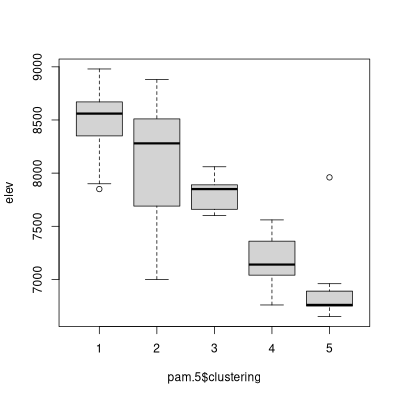
The $clustering values can be used just as the "cut" values from the
hierarchical cluster analysis before. For example,
boxplot(elev~pam.5$clustering)
The two algorithms can be compared as follows:
table(avg.5$clustering,pam.5$clustering)
     1  2  3  4  5
  1 30 52  4  1  0
  2  0  0  0 20  0
  3  0  0  0  0 14
  4  0  0 32  0  0
  5  2  0  4  0  1
match <- classmatch(avg.5,pam.5)
match
match
$tab
     pam.5
avg.5  1  2  3  4  5
    1 30 52  4  1  0
    2  0  0  0 20  0
    3  0  0  0  0 14
    4  0  0 32  0  0
    5  2  0  4  0  1

$pairs
   row column  n
1    1      2 52
2    4      3 32
3    1      1 30
4    2      4 20
5    3      5 14
6    1      3  4
7    5      3  4
8    5      1  2
9    1      4  1
10   5      5  1
The next table gives you the partial match at each step of filling out he
previous table.
$partial
 [1] 0.32500 0.52500 0.71250 0.83750 0.92500 0.95000 0.97500 0.98750
 [9] 0.99375 1.00000
$ord
     [,1] [,2] [,3] [,4] [,5]
[1,]    3    1    6    9    0
[2,]    0    0    0    4    0
[3,]    0    0    0    0    5
[4,]    0    0    2    0    0
[5,]    8    0    7    0   10
$combo
  [1]  3  3  3  3  1  3  1  1  3  1  1  1  3  1  1  3  1  1  1  1  1
 [22]  3  1  1  1  3  1  1  3  3  1  3  1  3  3  1  1  1  3  1  6  1
 [43]  1  1  1  1  1  3  1  1  1  1  1  1  1  3  1  1  3  3  3  3  3
 [64]  3  3  3  1  3  3  1  4  1  1  9  1  1  1  1  1  6  6  1  1  1
 [85]  3  3  1  5  5  5  5  5  5  5  5  5  5  5  5  5  5  2  2  2  2
[106]  2  2  2  2  2  2  2  2  2  2  2  2  2  2  2  2  2  2  2  2  2
[127]  2  2  2  2  2  6  7  7  7  7 10  8  2  2  8  4  4  4  4  4  4
[148]  4  4  4  4  4  4  4  4  4  4  4  4  4

attr(,"class")
[1] "classmatch"
attr(,"type")
[1] "full"
New Non-Hierachical Cluster Algorithms
Roberts (2015) introduced two new non-hierarchical algorithms called
optpart() and optsil. They had been in package
optpart for many years but never published.
optpart() and optsil are, like K-means, re-allocation
algorithms. This means you start off with an initial partition, and then
iteratively reassign sample units from one cluster to another to optimize a
goodness-of-clustering criterion. Not surprisingly, optpart()
optimizes the partana ratio, and optsil() optimizes silhouette widths.
optpart() and optsil can be run in either of two approaches:
(1) you can start with a random configuration, or (2) you can start with the
results of another cluster analysis and "polish" the results. If starting from
a random configuration, you probably want to start from numerous starts and keep
the best results. Here's an example with optpart()
opt.5 <- optpart(5,dis.bc)
summary(opt.5)
Number of clusters =  5

 1  2  3  4  5
12 14 38 92  4

           [,1]       [,2]       [,3]       [,4]       [,5]
[1,] 0.44024149 0.04602221 0.04753422 0.09648594 0.01069798
[2,] 0.04602221 0.42732677 0.08550955 0.01790267 0.04115028
[3,] 0.04753422 0.08550955 0.40820806 0.05513161 0.07337579
[4,] 0.09648594 0.01790267 0.05513161 0.36012116 0.06023967
[5,] 0.01069798 0.04115028 0.07337579 0.06023967 0.21904762

Ratio of Within-cluster similarity/Among-cluster similarity =  6.528 in 37
iterations
opt.5 <- bestopt(dis.bc,5,50)
Ratios for respective optparts
 [1] 6.528 6.376 6.528 6.376 6.528 6.528 6.528 6.376 6.528 6.528 6.528
[12] 6.528 6.528 6.382 6.528 6.528 6.528 6.528 6.528 6.376 6.528 6.528
[23] 6.528 6.528 6.528 6.528 6.528 6.528 6.528 6.528 6.528 6.528 6.528
[34] 6.376 6.376 6.528 6.528 6.528 6.528 6.528 6.528 6.528 6.376 6.528
[45] 6.528 6.528 6.528 6.528 6.528 6.528

Choosing #  25  ratio =  6.528
fb.5 <- slice(hcl.fb,5)
summary(partana(fb.5,dis.bc))
Number of clusters =  5

 1  2  3  4  5
31 45 32 14 38

           [,1]       [,2]       [,3]       [,4]       [,5]
[1,] 0.50286049 0.33445898 0.10643014 0.01414965 0.04821295
[2,] 0.33445898 0.53288949 0.16025466 0.01512236 0.04832595
[3,] 0.10643014 0.16025466 0.24271388 0.04331102 0.07499580
[4,] 0.01414965 0.01512236 0.04331102 0.42732677 0.08179415
[5,] 0.04821295 0.04832595 0.07499580 0.08179415 0.37590195

Ratio of Within-cluster similarity/Among-cluster similarity =  3.872
opt.fb <- optpart(fb.5,dis.bc)
Number of clusters =  5

 1  2  3  4  5
 4 92 12 14 38

           [,1]       [,2]       [,3]       [,4]       [,5]
[1,] 0.21904762 0.06023967 0.01069798 0.04115028 0.07337579
[2,] 0.06023967 0.36012116 0.09648594 0.01790267 0.05513161
[3,] 0.01069798 0.09648594 0.44024149 0.04602221 0.04753422
[4,] 0.04115028 0.01790267 0.04602221 0.42732677 0.08550955
[5,] 0.07337579 0.05513161 0.04753422 0.08550955 0.40820806

Ratio of Within-cluster similarity/Among-cluster similarity =  6.528 in 37
iterations
The default plot() for anoptpat() is of course a partana plot.
There is, however, third panel showing the progress of the optimization, show
here for the opt.fb result.
 optsil() can be run like optpart(). To generate a
five-cluster optsil do
optsil() can be run like optpart(). To generate a
five-cluster optsil do
sil.5 <- optsil(5,dis.bc,maxitr=250)
sil.5
$clustering
  [1] 3 3 3 3 3 3 3 3 3 3 3 3 3 3 3 3 3 3 3 3 3 3 3 3 3 3 3 3 3 3 3 3
 [33] 3 3 3 3 3 3 3 3 3 3 3 3 3 3 3 3 3 3 3 3 3 3 3 3 3 3 3 3 3 3 3 3
 [65] 3 3 3 3 3 3 2 3 3 1 3 3 3 3 3 4 4 3 3 3 3 3 3 5 5 5 5 5 5 2 2 5
 [97] 5 5 5 2 2 4 4 4 4 4 4 4 4 4 4 4 4 4 4 4 4 4 4 4 4 4 4 4 4 4 4 4
[129] 4 4 4 2 4 2 4 4 2 2 4 4 2 1 1 1 1 1 1 1 1 1 1 1 1 1 1 1 1 1 1 1

$sils
  [1] -0.0383837682 -0.0360490476 -0.0340548649 -0.0320981517
  [5] -0.0304199390 -0.0287459436 -0.0273244130 -0.0259370161
  [9] -0.0245875431 -0.0232583180 -0.0217805101 -0.0201710721
        .             .             .             .
        .             .             .             .
        .             .             .             .
[157]  0.2963449791  0.2989026435  0.3013503421  0.3035480820
[161]  0.3051924764  0.3070876618  0.3094570117  0.3109986270
[165]  0.3117793881  0.3121004686  0.3122590125  0.3126651665

$numitr
[1] 168

attr(,"class")
[1] "optsil"     "clustering"
attr(,"call")
optsil.default(x = 5, dist = dis.bc, maxitr = 250)
attr(,"timestamp")
[1] "Mon Mar 29 03:50:35 2021"
plot(silhouette(sil.5,dis.bc))
 optsil() can be slow to converge. In this case I specified a maximum
of 250 iterations and it ran for 168. Often the best idea is to start
optsil() from another cluster solution as the initial conditions.
optsil() can be slow to converge. In this case I specified a maximum
of 250 iterations and it ran for 168. Often the best idea is to start
optsil() from another cluster solution as the initial conditions.
sil.fb.5 <- optsil(fb.5,dis.bc)
sil.fb.5
$clustering
  [1] 1 1 1 1 2 1 2 2 1 2 2 2 1 2 2 1 2 2 2 2 2 1 1 2 2 1 2 2 1 1 2 1
 [33] 2 1 1 2 2 2 1 2 2 2 2 2 2 1 2 1 2 2 2 2 2 2 2 1 2 2 1 1 1 1 1 1
 [65] 1 1 2 1 1 2 3 2 2 3 2 2 2 2 2 5 5 2 2 2 1 1 2 4 4 4 4 4 4 4 4 4
 [97] 4 4 4 4 4 5 5 5 5 5 5 5 5 5 5 5 5 5 5 5 5 5 5 5 5 5 5 5 5 5 5 5
[129] 5 5 5 1 5 1 5 5 1 1 5 5 1 3 3 3 3 3 3 3 3 3 3 3 3 3 3 3 3 3 3 3

$sils
 [1] 0.2537863 0.2560616 0.2573747 0.2585516 0.2595028 0.2602953
 [7] 0.2608121 0.2618873 0.2625571 0.2629374 0.2635494 0.2641968
[13] 0.2645527 0.2650535 0.2655142 0.2655312

$numitr
[1] 16

attr(,"class")
[1] "optsil"     "clustering"
attr(,"call")
optsil.default(x = fb.5, dist = dis.bc)
attr(,"timestamp")
[1] "Mon Mar 29 04:00:18 2021"
par(mfrow=c(1,2))
plot(silhouette(fb.5,sdis.bc))
plot(silhouette(sil.fb.5,dis.bc))
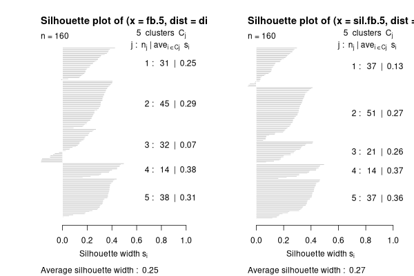 You can see that optsil() improved the silhouette width from 0.25 to
0.27. That's not great.
You can see that optsil() improved the silhouette width from 0.25 to
0.27. That's not great.
sil.opt.5 <- optsil(opt.5,dis.bc)
par(mfrow=c(1,2))
plot(silhouette(opt.5.dis.bc))
plot(silhouette(sil.opt.5.is.bc))
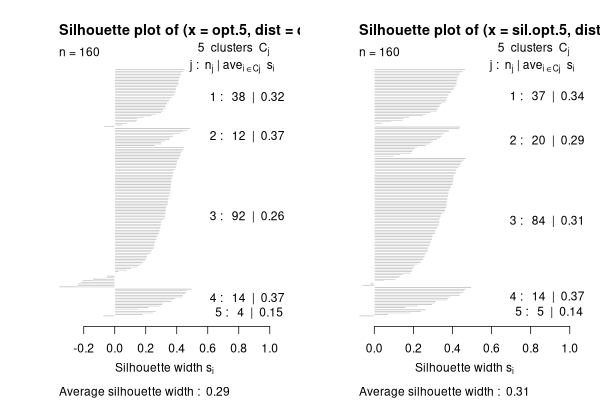 .
That's a littlr better.
.
That's a littlr better.
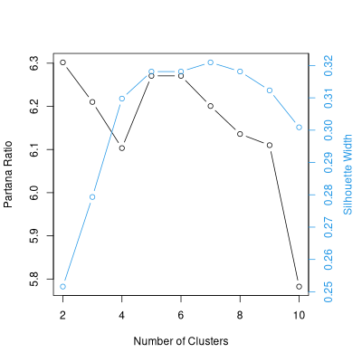
Using stride()
It's possible to use the stride function with optpart() or
. With optpart() you can proceed directly, by passing
a dissimilarity matrix and the argument "type='optpart'"
opt.2.10 <- stride(2:10,dis.bc,type='opt')
Ratios for respective optparts
 [1] 6.445 6.445 6.445 6.445 6.445 6.445 6.445 6.445 6.445 6.445

Choosing #  9  ratio =  6.445
Ratios for respective optparts
 [1] 6.286 6.404 6.278 6.286 6.286 6.278 6.286 6.546 6.278 6.286
     .     .     .     .     .     .     .    .    .    .     .
     .     .     .     .     .     .     .    .    .    .     .
     .     .     .     .     .     .     .    .    .    .     .
Choosing #  6  ratio =  6.534
Ratios for respective optparts
 [1] 4.488 6.534 6.534 4.481 6.534 4.485 4.307 6.534 6.534 4.473

Choosing #  8  ratio =  6.534
 With optsil you "polish" an existing stride.
sil.2.10 <- optsil(opt.2.10,dis.bc)
plot(sil.2.10,dis.bc)
 As an alternative, here's a polish of the average linkage result.
avg.sil.2.10 <- optsil(avg.2.10,dis.bc)
plot(avg.sil.2.10,dis.bc)
References
Aho, K., D.W. Roberts, and T.W.Weaver. 2008. Using geometric and
non-geometric internal evaluators to compare eight vegetation
classification methods. J. Veg. Sci. 19:549-562.
Kaufman, L. and P.J. Rousseeuw. Finding Groups in Data: An Introduction to
Cluster Analysis.
Lance, G.N., and W.T. Williams (1966). A General Theory of
Classificatory Sorting Strategies, I. Hierarchical Systems.
Computer J. 9:373-380.
Legendre, P. and L. Legendre (1998). Numerical Ecology.
Elsevier.
Lengyel, A., D.W. Roberts and Z. Botta-Dukat. 2021. Comparison of
silhouette‐based reallocation methods for vegetation classification. J. Veg.
Sci. 2021;32:e12984 https://doi.org/10.1111/jvs.12984
Maechler, M., Rousseeuw, P., Struyf, A., Hubert, M., Hornik,
K.(2019). cluster: Cluster Analysis Basics and Extensions. R package
version 2.1.0
Roberts, D.W. 2015. Vegetation classification by two new iterative reallocation
optimization algorithms. Plant Ecol. Vol. 216(5):741-758.
Rousseeuw, P.J. (1987) Silhouettes: A graphical aid to the interpretation and
validation of cluster analysis. J. Comput. Appl. Math. (20):53-65.
Library optpart
Library optpart is available at CRAN
Miscellaneous Scripts
const <- function (comm, clustering, minval = 0, show = minval, digits = 2,
    sort = FALSE, spcord = NULL)
{
    if (missing(clustering)) {
        const <- apply(comm > 0, 2, sum)/nrow(comm)
        const <- const[const >= minval]
        const <- data.frame(const)
        names(const) <- deparse(substitute(comm))
        return(round(const, digits))
    }
    else if (is.logical(clustering)) {
        comm <- comm[clustering, ]
        const <- apply(comm > 0, 2, sum)/nrow(comm)
        const <- const[const >= minval]
        const <- data.frame(const)
        names(const) <- deparse(substitute(clustering))
        return(round(const, digits))
    }
    clustering <- clustify(clustering)
    if (length(table(clustering)) == 1) {
        const <- apply(comm > 0, 2, sum)/nrow(comm)
        const <- const[const >= minval]
        const <- data.frame(const)
        return(round(const, digits))
    }
    else {
        res <- matrix(0, nrow = ncol(comm), ncol = length(levels(clustering)))
        x <- apply(comm, 2, function(x) {
            tapply(x > 0, clustering, sum)
        })
        y <- as.numeric(table(clustering))
        res <- x/y
        keep <- as.logical(apply(res, 2, max) >= minval)
        res <- res[, keep]
        tmp <- as.data.frame(t(res))
        row.names(tmp) <- names(comm)[keep]
        if (!is.null(spcord)) {
            tmp <- tmp[rev(order(spcord[keep])), ]
        }
        tmp <- format(round(tmp, digits = digits))
        tmp[tmp < show] <- substring(" .  ", 1, digits + 2)
        names(tmp) <- attr(clustering, "levels")
        attr(tmp, "call") <- match.call()
        attr(tmp, "timestamp") <- date()
        if (sort) {
            print(tmp)
            repeat {
                plots <- readline(" enter the species: ")
                if (plots == "") {
                  break
                }
                else {
                  pnt <- readline(" in front of        : ")
                }
                for (i in (strsplit(plots, ",")[[1]])) {
                  ord <- 1:nrow(tmp)
                  x <- match(i, row.names(tmp))
                  if (!is.na(x)) {
                    z <- ord[x]
                    ord <- ord[-x]
                    y <- match(pnt, row.names(tmp))
                    if (!is.na(y)) {
                      if (y > 1) {
                        first <- ord[1:(y - 1)]
                        last <- ord[y:length(ord)]
                        ord <- c(first, z, last)
                      }
                      else {
                        last <- ord[y:length(ord)]
                        ord <- c(z, last)
                      }
                      tmp <- tmp[ord, ]
                      print(tmp)
                    }
                    else {
                      print(paste("species", pnt, "does not exist"))
                    }
                  }
                  else {
                    print(paste("species", i, "does not exist"))
                  }
                }
            }
            return(tmp)
        }
    }
    return(tmp)
}
importance <- function (comm, clustering, minval = 0, digits = 2, show = minval,
    sort = FALSE, typical = TRUE, spcord, dots = TRUE)
{
    if (missing(clustering)) {
        impt <- apply(comm, 2, sum)/nrow(comm)
        impt <- impt[impt >= minval]
        impt <- data.frame(impt)
        names(impt) <- deparse(substitute(comm))
        return(round(impt, digits))
    }
    else if (is.logical(clustering)) {
        comm <- comm[clustering, ]
        impt <- apply(comm, 2, sum)/nrow(comm)
        impt <- impt[impt >= minval]
        impt <- data.frame(impt)
        names(impt) <- deparse(substitute(clustering))
        return(round(impt, digits))
    }
    clustering <- clustify(clustering)
    if (length(table(clustering)) == 1) {
        impt <- apply(comm, 2, sum)/nrow(comm)
        impt <- impt[impt >= minval]
        impt <- data.frame(impt)
        return(round(impt, digits))
    }
    else {
        res <- matrix(0, nrow = ncol(comm), ncol = length(levels(clustering)))
        x <- apply(comm, 2, function(x) {
            tapply(x, clustering, sum)
        })
        if (typical) {
            y <- apply(comm, 2, function(x) {
                tapply(x > 0, clustering, sum)
            })
        }
        else {
            y <- apply(comm, 2, function(x) {
                tapply(x >= 0, clustering, sum)
            })
        }
        y[x == 0] <- 1
        res <- x/y
        keep <- as.logical(apply(res, 2, max) >= minval)
        res <- res[, keep]
        tmp <- as.data.frame(t(res))
        row.names(tmp) <- names(comm)[keep]
        if (!missing(spcord)) {
            tmp <- tmp[rev(order(spcord[keep])), ]
        }
        if (dots) {
            tmpx <- format(round(tmp, digits = digits))
            tmpx[tmp < show] <- substring(" .  ", 1, nchar(tmpx[1,
                1]))
            print(tmpx)
        }
        if (sort) {
            cat("\nConstancy Table\n\n")
            print(tmp)
            repeat {
                plots <- readline(" enter the species: ")
                if (plots == "") {
                  break
                }
                else {
                  pnt <- readline(" in front of        : ")
                }
                for (i in (strsplit(plots, ",")[[1]])) {
                  ord <- 1:nrow(tmp)
                  x <- match(i, row.names(tmp))
                  if (!is.na(x)) {
                    ord <- ord[-x]
                    y <- match(pnt, row.names(tmp[ord, ]))
                    if (!is.na(y)) {
                      if (y == 1) {
                        ord <- c(x, ord)
                      }
                      else {
                        first <- ord[1:(y - 1)]
                        last <- ord[y:length(ord)]
                        ord <- c(first, x, last)
                      }
                      tmp <- tmp[ord, ]
                      print(tmp)
                    }
                    else {
                      print(paste("species", pnt, "does not exist"))
                    }
                  }
                  else {
                    print(paste("species", i, "does not exist"))
                  }
                }
            }
            attr(tmp, "call") <- match.call()
            attr(tmp, "comm") <- deparse(substitute(comm))
            return(tmp)
        }
    }
}
concov <- function (comm, clustering, digits = 1, width = 5, typical = TRUE,
    thresh = 10)
{
    if (missing(clustering)) {
        const <- apply(comm > 0, 2, sum)/nrow(comm)
        keep <- const >= thresh/100
        impt <- apply(comm, 2, sum)/nrow(comm)
        a <- formatC(as.numeric(const) * 100, width = 2, format = "d")
        b <- formatC(as.numeric(impt), width = width, digits = digits,
            format = "f")
        tmp <- NULL
        tmp <- cbind(tmp, paste(a, "(", b, ")", sep = ""))
        tmp <- tmp[keep]
        tmp <- data.frame(tmp)
        row.names(tmp) <- names(comm)[keep]
        attr(tmp, "call") <- match.call()
        attr(tmp, "comm") <- deparse(substitute(comm))
        attr(tmp, "timestamp") <- date()
        return(tmp)
    } else if (is.logical(clustering)) {
        comm <- comm[clustering, ]
        comm <- comm[, apply(comm > 0, 2, sum) > 0]
        x <- apply(comm > 0, 2, sum)
        y <- apply(comm, 2, sum)/x
        x <- x/nrow(comm)
        keep <- apply(as.matrix(x), 1, max) >= thresh/100
        a <- formatC(as.numeric(x) * 100, width = 2, format = "d")
        b <- formatC(as.numeric(y), width = width, digits = digits,
            format = "f")
        tmp <- NULL
        tmp <- cbind(tmp, paste(a, "(", b, ")", sep = ""))
        tmp <- tmp[keep]
        tmp <- data.frame(tmp)
        row.names(tmp) <- names(comm)[keep]
        names(tmp) <- deparse(substitute(clustering))
        attr(tmp, "call") <- match.call()
        attr(tmp, "comm") <- deparse(substitute(comm))
        attr(tmp, "clustering") <- clustering
        attr(tmp, "timestamp") <- date()
        return(tmp)
    }
    clustering <- clustify(clustering)
    if (length(table(clustering))==1)  {
        const <- apply(comm > 0, 2, sum)/nrow(comm)
        keep <- const >= thresh/100
        impt <- apply(comm, 2, sum)/nrow(comm)
        a <- formatC(as.numeric(const) * 100, width = 2, format = "d")
        b <- formatC(as.numeric(impt), width = width, digits = digits,
            format = "f")
        tmp <- NULL
        tmp <- cbind(tmp, paste(a, "(", b, ")", sep = ""))
        tmp <- tmp[keep]
        tmp <- data.frame(tmp)
        row.names(tmp) <- names(comm)[keep]
        names(tmp) <- deparse(substitute(clustering))
        attr(tmp, "call") <- match.call()
        attr(tmp, "comm") <- deparse(substitute(comm))
        attr(tmp, "clustering") <- clustering
        attr(tmp, "timestamp") <- date()
        return(tmp)
    } else {
        levels <- levels(clustering)
        clustering <- as.integer(clustering)
        x <- const(comm, clustering)
        y <- importance(comm, clustering, typical = typical)
        tmp <- NULL
        keep <- apply(as.matrix(x), 1, max) >= thresh/100
        for (i in 1:length(table(clustering))) {
            a <- formatC(as.numeric(x[, i]) * 100, width = 2,
                format = "d")
            b <- formatC(as.numeric(y[, i]), width = width, digits = digits,
                format = "f")
            tmp <- cbind(tmp, paste(a, "(", b, ")", sep = ""))
        }
        tmp <- tmp[keep, ]
        tmp <- data.frame(tmp)
        row.names(tmp) <- names(comm)[keep]
        names(tmp) <- levels
        attr(tmp, "call") <- match.call()
        attr(tmp, "comm") <- deparse(substitute(comm))
        attr(tmp, "clustering") <- clustering
        attr(tmp, "timestamp") <- date()
        return(tmp)
    }
    tmp
}
remos <-  function(d,gr,lim=-0.001,method=c(1,2),
                 return.partitions=FALSE,max.iter=Inf)
{
  # auth: Attila Lengyel
  gr_new <- gr
  o <-  -1
  z <- 1
  dw <- 1
  w <- u <- y <- vector('numeric')
  W <- matrix(NA, nrow=length(gr), ncol=0)
  parts <- vector('numeric')
  while(o < lim)  {
    SIL <- cluster::silhouette(gr_new,d)
    orig <- SIL[,1]
    neig <- SIL[,2]
    width <- SIL[,3]
    W <- cbind(W,width)
    if(method==1) worst <- which.min(width)
    if(method==2) worst <- which(width < lim)
    if(z > 1) dw <- as.vector(colSums((W-width)^2)[-z])
    o <- min(width)
    if(o < lim) {
     gr_new[worst] <- neig[worst]
    }
    y[z] <- o
    u[z] <- sum(width<0)
    w[z] <- abs(sum(width[width<0]))
    parts <- cbind(parts,gr_new)
    if(any(dw==0))   o <- lim+1
    if(z==max.iter) o <- lim+1
    z <- z+1
    }
  fin1 <- u==min(u)
  fin2 <- w==min(w[fin1]) & fin1
  gr_final <- parts[,fin2]

  if(return.partitions==TRUE) result <- list(gr_final,parts,y,u,w)
  if(return.partitions==FALSE) result <- list(gr_final,y,u,w)
  return(result)
}