To calculate a CCA, select those environmental variables you have reason to believe are important, and enter them into the cca() function in formula notation, just like we did for GLMs and GAMS. The full taxon matrix goes on the left-hand side of the equation, with selected environmental variables on the right.
attach(site)
cca.1 <- cca(bryceveg~elev+slope+av)
cca.1
Call: cca(formula = bryceveg ~ elev + slope + av)

              Inertia Proportion Rank
Total         10.8656     1.0000
Constrained    0.6976     0.0642    3
Unconstrained 10.1680     0.9358  147
Inertia is mean squared contingency coefficient

Eigenvalues for constrained axes:
  CCA1   CCA2   CCA3
0.5194 0.1110 0.0671

Eigenvalues for unconstrained axes:
   CA1    CA2    CA3    CA4    CA5    CA6    CA7    CA8
0.6912 0.5571 0.5278 0.4311 0.3752 0.3487 0.2900 0.2605
(Showed only 8 of all 147 unconstrained eigenvalues)
In this particular example, the CCA was not very successful. Only 0.6975/10.8656 or 0.064 of the total variability was captured in the CCA. Clearly, the weighted regression step was not very successful at capturing the variability in vegetation composition, but after glm() and gam() we should not be too surprised.
The next set of lines gives the eigenvalues associated with the projection. The top line gives the "constrained" eigenvalues. Because we only had three variables in our environmental dataframe we can only have three constrained eigenvalues. The three values sum to 0.69755. so
Plotting the CCA
To plot your results, use the plot() function as follows:
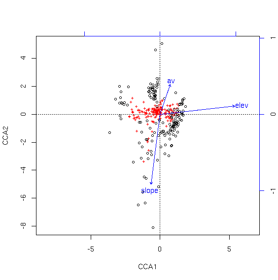
As for CA, the species are shown as red crosses and samples as black circles. In this analysis, the first axis is associated with increasing elevation, while the second axis is associated with decreasing slope and increasing aspect value (av).
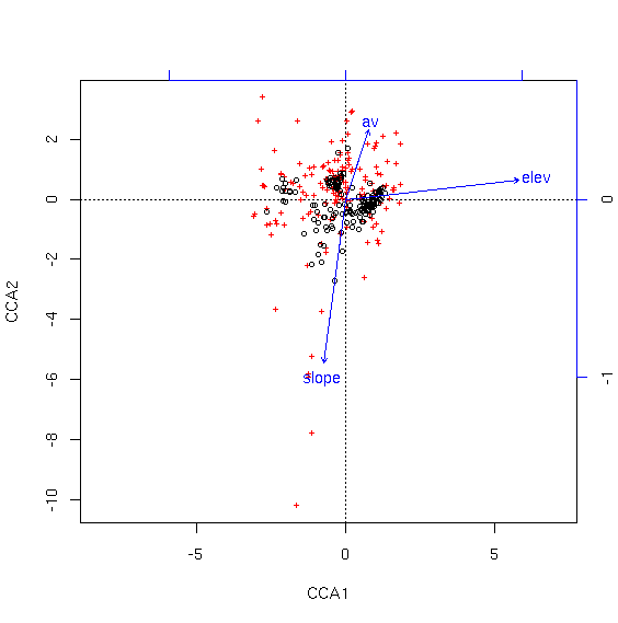
As you can see, the species are pretty well condensed in the center of the ordination. To get a better look, we can specify "scaling=1" to mean "samples as weighted averages of the species."
Package vegan supplies a number of graphing functions for ordiplots, including points() and identify(). We can use the identify() function to identify specific samples or species. Depending on whether you want a clearer picture of samples of species, you can plot using the appropriate scaling, and then use the identification functions with the same scaling.
cca1.plot <- plot(cca.1)
identify(cca1.plot,what='sites')
points(cca1.plot,what='sites',bryceveg$arcpat>0,col=3)
cca2.plot <- plot(cca.1,scaling=1)
identify(cca2.plot,what='species')
Adding Categorical Variables to the Analysis
If you are using the "formula" version of cca() (as we have been doing), then you can add categorical variables to the formula just as we did for GLMs and GAMS before. As an example, we can add topographic position to our model.cca.3 <- cca(bryceveg~elev+slope+av+pos) cca.3
Call: cca(formula = bryceveg ~ elev + slope + av + pos)

              Inertia Proportion Rank
Total         10.8656     1.0000
Constrained    1.1994     0.1104    7
Unconstrained  9.6662     0.8896  147
Inertia is mean squared contingency coefficient

Eigenvalues for constrained axes:
  CCA1   CCA2   CCA3   CCA4   CCA5   CCA6   CCA7
0.5268 0.2705 0.1292 0.0858 0.0723 0.0638 0.0510

Eigenvalues for unconstrained axes:
   CA1    CA2    CA3    CA4    CA5    CA6    CA7    CA8
0.6105 0.5365 0.4349 0.4074 0.3525 0.3274 0.2727 0.2598
(Showed only 8 of all 147 unconstrained eigenvalues)
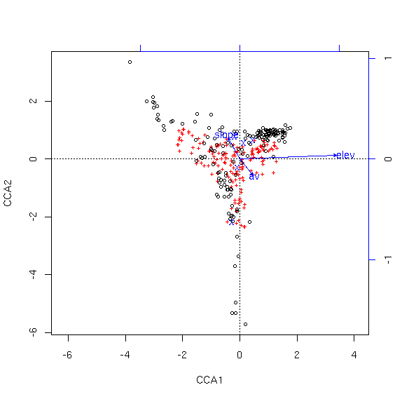
Notice how different this plot is from the first. While the total variability explained did not increase very much (and it can't go down with an increase of degrees of freedom), regressing the vegetation against topographic position in addition to the other variables results in a quite different perspective on the variability. Each possible topographic position is plotted at the centroid of the samples of that type, shown as an "X". To find out which one is which, look at last element of the summary of the cca object.
     .               .            .
     .               .            .
     .               .            .
Centroids for factor constraints

                 CCA1    CCA2    CCA3    CCA4    CCA5     CCA6
posbottom    -0.27212 -2.2070 -0.2082 -0.6002  0.7309  0.08555
poslow_slope -0.08944 -0.3111  0.7894  0.7438 -1.4639 -0.11783
posmid_slope  0.13114  0.5434 -0.1861  0.7238  0.7434  0.33647
posridge      0.45090  0.6428  0.6320 -0.6593  0.8699 -0.66962
posup_slope  -0.19154  0.7557 -0.8329 -1.6023 -0.7748 -0.23554
Discussion
CCA is overwhelmingly the most commonly used multivariate analysis in ecology. As an eigenanalysis it shares some of the benefits and shortcomings of eigenvector approaches. In contrast to PCA, it uses a Chi-square distance matrix rather than correlation/covariance. This solves the problem of treating joint absences as positive correlation, and is an improvement. On the other hand, as a true distance, it shares the problem of spurious "information" when two sites have no species in common, where their distance is a function of their productivity, rather than a constant. Finally, it assumes the the modes of species relate linearly to the environmental variables employed in the analysis. CCA has proven effective in an enormous number of studies, and is the first choice of most practicing ecologists.Ancillary Functions
The cca() function as implemented in package vegan employs the standard R step-wise fitting functions (add1(), drop1(), etc.). vegan author Jari Oksanen comments"The functions find statistics that resemble ‘deviance’ and ‘AIC’ in constrained ordination. Actually, constrained ordination methods do not have a log-Likelihood, which means that they cannot have AIC and deviance. Therefore you should not use these functions, and if you use them, you should not trust them. If you use these functions, it remains as your responsibility to check the adequacy of the result."
The function below does not make use of log-likelihood directly, but rather employs a rather brutish permutation approach and tests whether adding a variable explains more inertia than expected at random. Nonetheless, I'm sure Jari disapproves and I include it here for whatever good it might serve.
The argument start must be either NULL, a single continuous variable, or a data.frame. the argument addmust be a data.frame of variables to consider adding to the model. Variable must be continuous variables (i.e. not factors).
Baseline =  0
  variable  delta_eig p_val
1     elev 0.50503824  0.01
2    slope 0.11086016  0.05
3       av 0.08184252  0.19
Baseline =  0.5050382
  variable  delta_eig p_val
1    slope 0.11530671  0.11
2       av 0.07753032  0.13
step.cca <- function (taxa,start,add,numitr=99)
{
    perm.cca <- function(taxa,start,add,numitr) {
        rndeig <- rep(0,numitr)
        if (!is.null(start)) {
            for (i in 1:numitr) {
                tmp <- data.frame(start,sample(add,replace=FALSE))
                tmp2 <- cca(taxa,tmp)
                rndeig[i] <- sum(tmp2$CCA$eig)
            }
        }
        else {
            for (i in 1:numitr) {
                tmp <- data.frame(sample(add,replace=FALSE))
                tmp2 <- cca(taxa,tmp)
                rndeig[i] <- sum(tmp2$CCA$eig)
            }
        }
        return(rndeig)
    }

    res <- data.frame(names(add),rep(NA,ncol(add)),rep(NA,ncol(add)))
    names(res) <- c('variable','delta_eig','p_val')
    for (i in 1:ncol(add)) {
        if (!any(is.na(add[,i]))) {
            if (!is.null(start)) tmp <- data.frame(start,add[,i])
            else tmp <- add[,i]
            tmp <- cca(taxa,tmp)
            res[i,2] <- sum(tmp$CCA$eig)
        }
        rndeig <- perm.cca(taxa,start,add[,i],numitr)
        if (!is.null(start)) {
            full <- data.frame(start,add[,i])
            base <- cca(taxa,start)
            basval <- sum(base$CCA$eig)
        }
        else {
            full <- add[,i]
            basval <- 0
        }
        res[i,3] <- (sum(rndeig>=res[i,2])+1)/(numitr+1)
        res[i,2] <- res[i,2] - basval
    }
    cat(paste("Baseline = ", format(basval, 3), "\n"))
    print(res)
}


step.cap <- function (diss,start,add,numitr=99)
{
    perm.capscale <- function(diss,start,add,numitr) {
        rndeig <- rep(0,numitr)
        if (!is.null(start)) {
            for (i in 1:numitr) {
                tmp <- data.frame(start,sample(add,replace=FALSE))
                tmp2 <- capscale(diss~.,data=tmp)
                rndeig[i] <- sum(tmp2$CCA$eig)
            }
        }
        else {
            for (i in 1:numitr) {
                tmp <- data.frame(sample(add,replace=FALSE))
                tmp2 <- capscale(diss~.,data=tmp)
                rndeig[i] <- sum(tmp2$CCA$eig)
            }
        }
        return(rndeig)
    }

    res <- data.frame(names(add),rep(NA,ncol(add)),rep(NA,ncol(add)))
    names(res) <- c('variable','delta_eig','p_val')
    for (i in 1:ncol(add)) {
        if (!any(is.na(add[,i]))) {
            if (!is.null(start)) tmp <- data.frame(start,add[,i])
            else tmp <- data.frame(add[,i])
            tmp <- capscale(diss~.,data=tmp)
            res[i,2] <- sum(tmp$CCA$eig)
        }
        rndeig <- perm.capscale(diss,start,add[,i],numitr)
        if (!is.null(start)) {
            full <- data.frame(start,add[,i])
            start <- data.frame(start)
            base <- capscale(diss~.,data=start)
            basval <- sum(base$CCA$eig)
        }
        else {
            full <- add[,i]
            basval <- 0
        }
        res[i,3] <- (sum(rndeig>=res[i,2])+1)/(numitr+1)
        res[i,2] <- res[i,2] - basval
    }
    cat(paste("Baseline = ", format(basval, 3), "\n"))
    print(res)
}