Up to this point we have generally been performing ordination analyses according to the protocol of:
With the exception of RDA (Lab 7), the configuration of the points in PCA, PCO, and NMDS ordinations has been completely determined by the vegetation compositional data. Alternatively, for CCA and DB-RDA the configuration of points is first calculated as a CA or PCO respectively, which is then subjected to weighted regression against environmental or experimental variables, keeping the fitted values of the regression as coordinates. Accordingly, CCA and DB-RDA are referred to as "constrained ordinations" as they constrain the values of the underlying ordination to achieve what is typically referred to as their "canonical" axes. FSO is the first technique that directly incorporates the environmental data into the calculation of the configuration.
The initial application of FSO to single variables bears more resemblance to the surface fitting routines we have employed so far than to the dimensional mapping routines. That is, when we calculate an FSO on elevation, for example, the result is an estimate of the relative elevation for each plot, based on its composition. If a variable is influential in determining or constraining the distribution of vegetation, then we ought to be able to estimate the value of that variable based on the composition. This is an approach called "calibration" by Ter Braak and colleagues (19xx). Whether or not the ordination achieves an efficient mapping from high-dimensional space to low dimensional space is a secondary consideration, and generally requires solving for multiple dimensions. All this is more easily understood by example.
The FSO is calculated with a function called fso(), which requires two arguments: a variable (or multiple variables in a formula or data.frame) and a similarity matrix. Because the convention in R is to work with dist objects, fso() automatically converts the dist object from dist(), dsvdis() or vegdist to a full similarity matrix as required. From our previous work with other methods, we have good reason to expect that elevation and slope may be important, so let's start with elevation.
First, let's get the fso package with the necessary functions. and then enter library(fso).
install.packages('fso')
library(fso)
As we have throughout the previous labs, we'll analyze the Bryce Canyon data. So, if you haven't already
library(labdsv)
data(bryceveg)
data(brycesite)
attach(brycesite)
dis.bc <- dsvdis(bryceveg,'bray/curtis')
fso() does its work silently. to examine the results, use
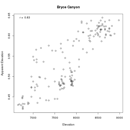
As you can see, the relationship between elevation and "apparent elevation" is pretty good, with a correlation of 0.83 (upper left corner). That means that on average we can predict the elevation of a sample from its composition fairly well. There are some interesting outliers, though, that bear looking into. How about slope?
slope.fso <- fso(slope,dis.bc)
plot(slope.fso,title="Bryce Canyon")
Hmmm. While a correlation of 0.35 is not too bad, the distribution leaves something to be desired. The problem is that the distribution of sample plots is not remotely uniform for slope, with many more plots on gentle slopes than steep. As a possible fix, we can try
slope.log.fso <- fso(log(slope+1),dis.bc)
plot(slope.log.fso)
Despite the emphasis on a priori concepts about the control of vegetation composition by environment it has proven helpful to write routines that facilitate rapid screening and analysis of a broad range of possible variables. fso() will accept a formula or dataframe as its first argument, and perform sequential FSOs on the variables. For example,
Fuzzy set statistics

  col variable         r            p         d
1   1     elev 0.8303255 0.000000e+00 0.6119908
2   3    slope 0.3495267 5.891172e-06 0.3208229
3   4   annrad 0.3050769 8.758970e-05 0.2255343
4   5   grorad 0.3013482 1.078098e-04 0.5811717
5   2       av 0.1402331 7.694954e-02 0.1985226

Correlations of fuzzy sets

             elev         av      slope     annrad     grorad
elev    1.0000000  0.5936768 -0.5018290 -0.7666193 -0.8255718
av      0.5936768  1.0000000 -0.6119128 -0.9184280 -0.5206253
slope  -0.5018290 -0.6119128  1.0000000  0.6292742  0.1255797
annrad -0.7666193 -0.9184280  0.6292742  1.0000000  0.7297448
grorad -0.8255718 -0.5206253  0.1255797  0.7297448  1.0000000
Finally, in the bottom matrix it presents a correlation matrix of the derived fuzzy sets.
To plot each of the variables in succession, simply enter
The estimated p-values are computed from a Normal approximation with the appropriate numbers of degrees of freedom. Nonetheless, in my experience they have proven somewhat problematic (slightly high type I error rate), and I have included a permutation-based statistic as an alternative. Essentially, the routine permutes the input vector (permute -1 times), calculates an FSO, and stores the correlation in a vector. The statistic reported is
grads.fso <- fso(~elev+av+slope+annrad+grorad,dis.bc,permute=1000)
summary(grads.fso)
Fuzzy set statistics

  col variable         r     p         d
1   1     elev 0.8303255 0.001 0.6119908
2   3    slope 0.3495267 0.001 0.3208229
3   4   annrad 0.3050769 0.001 0.2255343
4   5   grorad 0.3013482 0.001 0.5811717
5   2       av 0.1402331 0.064 0.1985226
| scaling | algorithm |
| 1 | no scaling, use actual mu values |
| 2 | relativize both fuzzy sets [0,1] |
| 3 | center and scale proportional to their correlation coefficient |
In either case, the regression step (and subsequent rescaling of the second axis to the residuals of the regression) is controlled by lm=.
To see the result, simple use the plot function.
Because in this case the two sets were not very strongly correlated, the second set retains a fairly broad range of mu values. For sets that are more strongly correlated, the Y axis may have a much more restricted range. How good a job does this mapping do? The dis= argument allows you to specify a dissimilarity/distance matrix to compare the ordination distances to. If specified, the values show up in the last plot.
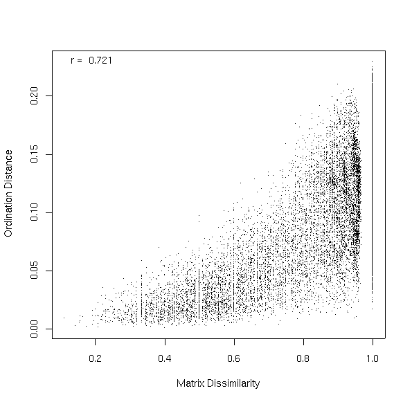
In this case, the correlation between ordination distances and dissimilarities in the original matrix is 0.721. Looking back to Lab 8, the PCO two-dimensional projection of the Bray/Curtis dissimilarity matrix achieved 0.788, so our three-dimensional FSO is almost as good as a PCO in terms of faithful representation of dissimilarities, and has the added benefit of an obvious ecological interpretation.
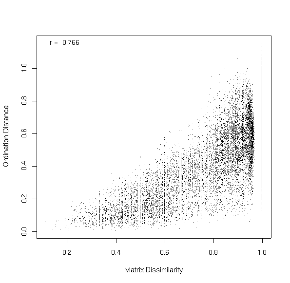
The alternative, using scaling=2 turns out slightly better.
grads2.mfso <- mfso(~elev+slope+grorad,dis.bc,scaling=2)
plot(grads2.mfso,dis.bc)
Slope and grorad is also an interesting combination.
mfso.2 <-mfso(~slope+grorad,dis.bc,scaling=2)
plot(mfso.2)
elev.fso.lm <- lm(elev.fso$mu~elev)
summary(elev.fso.lm)
Call:
lm(formula = elev.fso$mu ~ elev)

Coefficients:
              Estimate Std. Error t value Pr(>|t|)
(Intercept) -1.819e-01  3.856e-02  -4.717 5.23e-06 ***
elev         9.162e-05  4.892e-06  18.729  < 2e-16 ***
---
Signif. codes:  0  `***'  0.001  `**'  0.01  `*'  0.05  `.'  0.1  ` '  1

Residual standard error: 0.03801 on 158 degrees of freedom
Multiple R-Squared: 0.6894,     Adjusted R-squared: 0.6875
F-statistic: 350.8 on 1 and 158 degrees of freedom,     p-value:     0
Call:
lm(formula = elev.fso.res ~ grorad)


Coefficients:
             Estimate Std. Error t value Pr(>|t|)
(Intercept)  0.401664   0.078248   5.133 8.27e-07 ***
grorad      -0.002460   0.000479  -5.136 8.15e-07 ***
---
Signif. codes:  0  `***'  0.001  `**'  0.01  `*'  0.05  `.'  0.1  ` '  1

Residual standard error: 0.03519 on 158 degrees of freedom
Multiple R-Squared: 0.1431,     Adjusted R-squared: 0.1377
F-statistic: 26.38 on 1 and 158 degrees of freedom,     p-value: 8.148e-07
How about topographic position? We'll add it to growing season radiation to look for conditional significance. The R lm() routine handles categorical variables like pos without recoding, establishing contrasts to the first category.
Call:
lm(formula = elev.fso.res ~ grorad + pos)

Residuals:
       Min         1Q     Median         3Q        Max
-0.0665706 -0.0239119 -0.0006207  0.0232542  0.0939038

Coefficients:
               Estimate Std. Error t value Pr(>|t|)
(Intercept)   0.3714292  0.0816540   4.549 1.09e-05 ***
grorad       -0.0023628  0.0004907  -4.816 3.48e-06 ***
poslow_slope  0.0233538  0.0099608   2.345   0.0203 *
posmid_slope  0.0148793  0.0093715   1.588   0.1144
posridge      0.0165458  0.0113768   1.454   0.1479
posup_slope   0.0118876  0.0098836   1.203   0.2309
---
Signif. codes:  0  `***'  0.001  `**'  0.01  `*'  0.05  `.'  0.1  ` '  1

Residual standard error: 0.03499 on 154 degrees of freedom
Multiple R-Squared: 0.174,      Adjusted R-squared: 0.1472
F-statistic: 6.488 on 5 and 154 degrees of freedom,     p-value: 1.675e-05
Analysis of Variance Table

Response: elev.fso.res
           Df   Sum Sq  Mean Sq F value    Pr(>F)
grorad      1 0.032666 0.032666 26.6776 7.337e-07 ***
pos         4 0.007056 0.001764  1.4406    0.2232
Residuals 154 0.188566 0.001224
---
Signif. codes:  0  `***'  0.001  `**'  0.01  `*'  0.05  `.'  0.1  ` '  1
To look at the effects of soil depth, remembering from Lab 2 that soil depth is correlated with elevation, we need to correct for elevation first. We'll run the summary of the regression first to get the signs and coefficients and then the anova to check for sequential significance.
Call:
lm(formula = elev.fso.res ~ elev + depth)

Residuals:
      Min        1Q    Median        3Q       Max
-0.075054 -0.024821 -0.002617  0.020813  0.092883

Coefficients:
               Estimate Std. Error t value Pr(>|t|)
(Intercept)  -1.120e-02  3.683e-02  -0.304    0.761
elev         -1.016e-06  4.729e-06  -0.215    0.830
depthshallow  2.829e-02  5.839e-03   4.845 3.27e-06 ***
---
Signif. codes:  0  `***'  0.001  `**'  0.01  `*'  0.05  `.'  0.1  ` '  1

Residual standard error: 0.03325 on 142 degrees of freedom
Multiple R-Squared: 0.1467,     Adjusted R-squared: 0.1347
F-statistic:  12.2 on 2 and 142 degrees of freedom,     p-value: 1.285e-05
Analysis of Variance Table

Response: elev.fso.res
           Df   Sum Sq  Mean Sq F value    Pr(>F)
elev        1 0.001033 0.001033  0.9341    0.3354
depth       1 0.025951 0.025951 23.4743 3.274e-06 ***
Residuals 142 0.156981 0.001105
---
Signif. codes:  0  `***'  0.001  `**'  0.01  `*'  0.05  `.'  0.1  ` '  1
| dis | the dissimilarity/distance object | no default |
| start | the variables in the initial model as a data.frame | no default, can be NULL |
| add | the variables to consider for addition to the model as a data.frame | no default |
| numitr | the number of random permutations to use to calculate p-values | default = 100 |
| scaling | the scaling to use on MFSO (see above) | default = 1 |
Here's an example of step.mfso() in use
attach(brycesite)
step.mfso(dis.bc,start=NULL,add=data.frame(elev,slope,av,grorad,annrad))
Baseline =  0
  variable delta_cor p_val
1     elev 0.6119908  0.08
2    slope 0.3208229  0.66
3       av 0.1985226  0.90
4   grorad 0.5811717  0.08
5   annrad 0.2255343  0.82
Baseline =  0.6119908
  variable    delta_cor p_val
1    slope  0.101305309  0.01
2       av -0.001551554  0.98
3   grorad  0.050204388  0.01
4   annrad -0.002196274  1.00
Baseline =  0.7132961
  variable     delta_cor p_val
1       av -0.0014125421  0.96
2   grorad  0.0078175173  0.04
3   annrad -0.0009994769  0.99
step.mfso(dis.bc,start=data.frame(elev,slope),add=data.frame(av,grorad,annrad),
          numitr=1000)
Baseline =  0.7132961
  variable     delta_cor p_val
1       av -0.0014125421 0.906
2   grorad  0.0078175173 0.035
3   annrad -0.0009994769 0.993
The outcome of the step-wise function in this case gives us the same model we had analyzed above (elev then slope) with arguably a third dimension for grorad. To screen large numbers of variables it is sometimes advisable to set numitr=1 during the variable selection stage, and then put just the selected variable in the add data.frame for permutation testing.
We also have a primary gradient for slope which is nearly independent of the elevation gradient. Regressing the residuals of the slope FSO (not shown) only showed one statistically significant effect (annrad), such that sites with high annual radiation appeared to be slightly steeper than they really are. This appears to be because radiation is an asymmetric function of aspect, where level sites have radiation budgets more similar to south slopes than to north slopes.
We don't have sufficient climate data to tease apart the elevation effect; it combines both temperature and presumably precipitation, but we can't partition the two. It's an example of what Austin and Smith (19xx) would call a "complex gradient." The slope gradient is also probably best viewed as a complex gradient. The ecological characteristics of slope (apart from aspect effects ON slopes) is likely soil erosion and consequent soil texture effects. Steep slopes are likely to suffer from removal of fine-textured soil particles and run-off of precipitation, leading to drier sites than level sites at equivalent elevations.
FSO is thus useful for analysis of primary gradients, as well as nested secondary effects within primary gradients. The multi-FSO plots are nearly as efficient as PCO, with much more immediate ecological interpretation possible.
Roberts, D.W. 2008. Statistical analysis of multidimensional fuzzy set ordination. Ecology 89:1256-1260.
Roberts, D.W. 2009. Comparison of multidimensional fuzzy set ordination with CCA and DB-RDA. Ecology 90:2622-2634.
plot.fso <- function (x, which = "all", xlab = x$var, ylab = "mu(x)", title = "",
    r = TRUE, pch = 1, ...)
{
    if (class(x) != "fso") {
        stop("You must specify n object of class fso from fso()")
    }
    if (is.matrix(x$mu)) {
        if (which == "all") {
            for (i in 1:ncol(x$mu)) {
                if (is.na(x$r[i])) {
                  cat(paste("variable ", x$var[i], " has missing values \n"))
                }
                else {
                  plot(x$data[, i], x$mu[, i], xlab = xlab[i], ylab = ylab,
                    main = title)
                  if (r) {
                    ax <- min(x$data[, i])
                    ay <- max(x$mu[, i])
                    text(ax, ay, paste("r = ", format(x$r[i],
                      digits = 3)), pos = 4)
                  }
                }
                readline("\nHit Return for Next Plot\n")
            }
        }
        else if (is.numeric(which)) {
            for (i in which) {
                plot(x$data[, i], x$mu[, i], xlab = xlab[i], ylab = ylab,
                  main = title)
                if (r) {
                  ax <- min(x$data[, i])
                  ay <- max(x$mu[, i])
                  text(ax, ay, paste("r = ", format(x$r[i], digits = 3)),
                    pos = 4)
                }
                readline("\nHit Return for Next Plot\n")
            }
        }
        else {
            for (j in 1:ncol(x$mu)) {
                if (which == x$var[j])
                  plot(x$data[, j], x$mu[, j], xlab = xlab[j], ylab = ylab,
                    main = title)
                if (r) {
                  ax <- min(x$data[, j])
                  ay <- max(x$mu[, j])
                  text(ax, ay, paste("r = ", format(x$r[j], digits = 3)),
                    pos = 4)
                }
            }
        }
    }
    else {
        plot(x$data, x$mu, xlab = xlab, ylab = ylab, main = title)
        if (r) {
            ax <- min(x$data)
            ay <- max(x$mu)
            text(ax, ay, paste("r = ", format(x$r, digits = 3)),
                pos = 4)
        }
    }
}
surf.mfso <- function (ord, var, ax = 1, ay = 2, thinplate = TRUE, col = 2,
    labcex = 0.8, family = gaussian, gamma = 1, grid = 50, ...)
{
    if (!inherits(ord, "mfso"))
        stop("You must supply an object of class 'mfso'")
    if (missing(var)) {
        stop("You must specify a variable to surface")
    }
    x <- ord$mu[, ax]
    y <- ord$mu[, ay]
    if (any(is.na(var))) {
        cat("Omitting plots with missing values \n")
        x <- x[!is.na(var)]
        y <- y[!is.na(var)]
        var <- var[!is.na(var)]
    }
    if (is.logical(var)) {
        tvar <- as.numeric(var)
        if (thinplate)
            tmp <- gam(tvar ~ s(x, y), family = binomial, gamma = gamma)
        else tmp <- gam(tvar ~ s(x) + s(y), family = binomial,
            gamma = gamma)
    }
    else {
        if (thinplate)
            tmp <- gam(var ~ s(x, y), family = family, gamma = gamma)
        else tmp <- gam(var ~ s(x) + s(y), family = family, gamma = gamma)
    }
    new.x <- seq(min(x), max(x), len = grid)
    new.y <- seq(min(y), max(y), len = grid)
    xy.hull <- chull(x, y)
    xy.hull <- c(xy.hull, xy.hull[1])
    new.xy <- expand.grid(x = new.x, y = new.y)
    inside <- as.logical(pip(new.xy$x, new.xy$y, x[xy.hull],
        y[xy.hull]))
    fit <- predict(tmp, type = "response", newdata = as.data.frame(new.xy))
    fit[!inside] <- NA
    contour(x = new.x, y = new.y, z = matrix(fit, nrow = grid),
        add = TRUE, col = col)
    print(tmp)
    d2 <- (tmp$null.deviance - tmp$deviance)/tmp$null.deviance
    cat(paste("D^2 = ", formatC(d2, width = 4), "\n"))
    invisible(tmp)
}
dummify <- function (var)
{
    if (!is.factor(var)) stop('You must pass a factor variable')

    cols <- length(levels(var))
    out <- matrix(0,nrow=length(var),ncol=cols)
    for (i in 1:cols) {
        out[,i] <- var == levels(var)[i]
    }
    out <- data.frame(out)
    names(out) <- levels(var)
    out
}
ellip.mfso <- function (ord, overlay, ax = 1, ay = 2, cols = c(2, 3, 4, 5,
    6, 7), ltys = c(1, 2, 3), ...)
{
    if (class(ord) != "mfso")
        stop("You must pass an object of class mfso")
    require(cluster)
    if (inherits(overlay, c("partana", "pam", "clustering"))) {
        overlay <- overlay$clustering
        if (min(overlay) < 0 || (length(table(overlay)) != max(overlay))) {
            cat("WARNING: renumbering clusters to consecutive integers\n")
            overlay <- match(overlay, sort(unique(overlay)))
        }
    }
    else if (is.logical(overlay))
        overlay <- as.numeric(overlay)
    else if (is.factor(overlay))
        overlay <- as.numeric(overlay)
    pass <- 1
    layer <- 0
    lty <- ltys[pass]
    for (i in 1:max(overlay, na.rm = TRUE)) {
        x <- ord$mu[, ax][overlay == i & !is.na(overlay)]
        y <- ord$mu[, ay][overlay == i & !is.na(overlay)]
        pts <- chull(x, y)
        layer <- layer + 1
        if (layer > length(cols)) {
            layer <- 1
            pass <- min(pass + 1, length(ltys))
        }
        col <- cols[layer]
        lty = ltys[pass]
        x <- as.matrix(cbind(x[pts], y[pts]))
        elp <- ellipsoidhull(x)
        lines(predict(elp),col=col)
    }
}