CA can be calculated by a number of different algorithms. Due to the popularity of the analysis there are a number of different implementations of CA in R. A function called ca() is included in the mva library. The CoCoAn library includes CA as a special case of CCA (see Lab 12) in the function CAIV(), and the vegan library includes CA as a special case of DECORANA() or cca(see below). The method presented here is due to Legendre and Legendre (1998), who calculate CA as an eigenanalysis of a particular matrix.
Labs 6 and 7 describe eigenanalysis of a number of different matrices. PCA is specifically an eigenanalysis of a correlation or covariance matrix. PCO is an eigenanalysis of a broad variety of symmetric dissimilarity/distance matrices. CA is an eigenanalysis of a Chi-square distance matrix. A Chi-square distance matrix is defined by the deviation from expectation. Similar to the Chi-square statistic, it is defined as
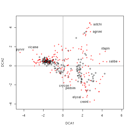
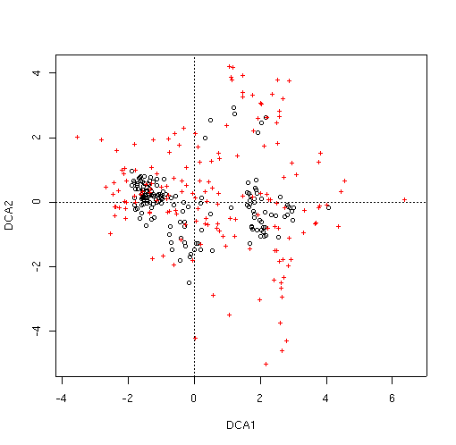
In contrast to the ordination methods we have employed so far, CA provides a configuration for species as well as sample plots in the ordination. That is, species centroids (the hypothetical mode of their distribution along the eigenvectors) can be plotted as well as the locations of the plots. This dual nature is one of the characteristics that first attracted ecologists to CA.
We can perform CA much as we did PCA in Lab 6, using the vegetation matrix (as opposed to a dissimilarity/distance matrix). LabDSV no longer has a ca() function, but you can paste in the function from the bottom of this lab here.
The LabDSV convention is to plot samples in black (as for PCA, PCO, and NMDS) and species in red (in a different symbol as well) as shown. CA is known to be sensitive to rare species and outlier plots, and what you see is an indication of that. One species (to be identified later) is an extreme outlier on the y axis, and since the x axis is scaled to maintain an aspect ratio of 1.0, condenses the plots and species along both axes. To identify the offending species, we can use the specid.ca() function. Similar to how we used identify() way back in Lab 1, specid.ca() works similarly. Call specid.ca() with an argument to specify the CA and the scaling, and optionally a vector of species names as follows.
We can identify sample plots with the LabDSV plotid.ca() function in the same way.
Programs like DECORANA (Hill and Gaugh, 1980) have options to "downweight" rare species to minimize the problem out species as outliers. One example of the problem is to identify the number of plots each species occurs in in the diagram. Back in Lab 1 we calculated the number of plots each species occurred in as spc.pres. Let's use that as the identifier.
plot(ca.1,scaling=1)
specid.ca(ca.1,scaling=1,spc.pres)
Many (but not all) of the species lying at extremes of the cloud are species that only occur once or a few times. Accordingly, while ca() doesn't have a rare species downweighting function, we can leave them out all together, using logical subscripts (see Lab 1 for a refresher if necessary).
The dispersion is a little better, but qualitatively it's pretty similar to before.
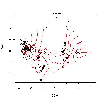
Similar to PCA, PCO, and NMDS, there are points() and surf.ca() functions for CA as well, all at th ebottom of this page. Often, you will want better dispersion of the sample plots before calculating the surface, and scaling type 2 will work better. For example, using elevation again
plot(ca.1,scaling=2)
surf.ca(ca.1,elev,scaling=2)
Family: gaussian
Link function: identity

Formula:
var ~ s(x) + s(y)

Estimated degrees of freedom:
 2.573253 4.742089   total =  8.315343

GCV score:  160641.8
D^2 =  0.6174
Because the CA plot program uses two colors already, the default for surf() for CA is to plot contours in green (col=3) to start. Despite the fact that the graph is not very interpretable visually, the D^2 square is not too bad (0.617 vs 0.870 for PCO). Surfaces for slope and aspect value (see Lab 8 are not very satisfactory either, despite reasonable D^2s. In fairness, the Bryce data set probably has too much beta-diversity for CA. Although less sensitive then PCA, CA also suffers when applied to high beta-diversity.
vegan has a different set of conventions than LabDSV, especially with respect to plotting, and it's probably just as well to cover them here. Oksanen is really a master with R, and his code reflects much greater finesse and a deeper immersion into R than LabDSV. It's indicative of R that there isn't just one way to do things, but that fairly strong conventions are beginning to emerge.
To produce an ordination with vegan, you simply call an ordination function like you did with LabDSV, storing the result in an ordination object. To plot the ordination, you can simply plot is, again like LabDSV. Generally, however, you will want to store the (invisible) result of the plot in another variable. This variable has class "ordiplot," and stores all the information about the plot, such as which axes were plotted, and the coordinates of sites and species on just those axes, not all. This greatly simplifies subsequent labeling and surfacing, as the routines now magically know which axes were plotted, as well as some other information. Let me give an example using decorana
library(vegan)                # if you haven't already
veg.dca <- decorana(veg)
veg.dca.plt <- plot(veg.dca)  # notice the assignment used with a plot function
Now, to identify species (for example) you use an identify function on the
ordiplot object, specifying either "species" or "sites".
By default, the identify function labels in black, but to get the LabDSV convention
of species in red, you could just do
With a little bit of practice, you'll get the hang of the vegan ordiplot
convention, and find it quite helpful. If you want to, you can look directly at the
ordiplot object.
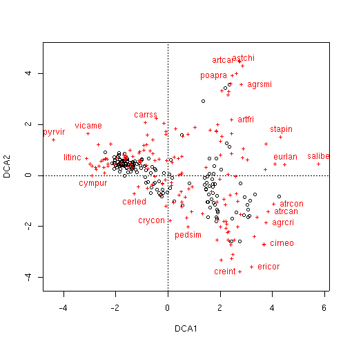
While the X axis has been stretched extraordinarily compared to CA, the species
near the edge are still basically the same. Again, in contrast to
ca(), decorana() DOES allow downweighting of rare species with
the weigh=TRUE argument. Let's see if it helps.
Unfortunately, the plots are even more congested than before, so it will be
difficult to get interpretations of the configuration. Fortunately, we don't have to
worry about this too much. the vegan library contains a function called
ordisurf which is similar to our previous surf function from LabDSV.
However, instead of overlaying the contours on the existing plot, it replots the sites
and then puts on the contours. In our case, this effectively spreads out the points.
Notice that we ordiplot the ordiplot object, not the decorana object. The
default action is to draw a new plot, so to put a second set of contours on, use
add=TRUE in your ordisurf command.
> ordisurf(dca.2.plt,slope,col=3,add=TRUE)
We can always resort to
re-plotting by hand when the canned routines don't so what we want.
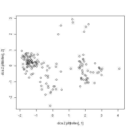
The dca.2.plt ordiplot object has the plot scores stored as
dca.2.plt$sites, so we can plot those on their own scale.
> ordisurf(dca.2,elev)
Family: gaussian
Link function: identity
Formula:
var ~ s(x) + s(y)
Estimated degrees of freedom:
6.858568 5.219111 total = 13.07768
GCV score: 117732.2
D^2 = 0.7369
The D^2 of 0.740 is not too bad (better than we got for PCA and PCO with
Euclidean or Manhattan distance, worse than PCO or NMDS with Bray/Curtis).
Slope and aspect values (not shown) are also better than PCA or PCO with
Euclidean distance, but worse than PCO with Bray/Curtis, but similar to NMDS.
While DECORANA was the ordination method of choice in the 70's and 80's, it was
severely criticized for some of the "detrending" algorithms. While they were
arguably inelegant (if not heavy-handed), empirically (as seen here) they were
regarded as a significant improvement on CA. Part of the reason that the
controversy died is that Canonical Correspondence Analysis (CCA) came along and
rendered many of the arguments moot. CCA is presented in Lab 10.
identify(veg.dca.plt,'species')
[1] 39 45 75 90 91 144 155 156 160 169
 identify(veg.dca.plt,'species',col=2)
veg.dca.plt
identify(veg.dca.plt,'species',col=2)
veg.dca.plt
$sites
           DCA1         DCA2
1   -1.80693591  0.516629756
2   -1.87728354  0.869333630
3   -1.67522711  0.855566371
4   -1.77212021  0.564803776
5   -1.83270809  0.509189062
6   -2.03194434  0.617906119
.         .            .
.         .            .
.         .            .
157 -0.42922861 -0.548282629
158 -0.76827770 -0.270540304
159 -0.21667241 -0.554282368
160 -0.35125690 -0.238909761

$species
                DCA1         DCA2
junost    2.90922011  1.025643152
ameuta   -2.60907005  0.355392235
arcpat   -2.27476065  0.343951025
arttri    3.45120077 -1.654125085
   .           .          .
   .           .          .
   .           .          .
towmin   -0.05610011  1.706885447
tradub    3.08098986  0.606207632
valacu   -0.78198398  1.189948147
vicame   -3.03292127  1.625904397

attr(,"class")
[1] "ordiplot"
Back to Ecology
The dispersion appears much better than we obtained with CA. Unlike
ca(), we don't have dual scalings for decorana; it calculates
similar to scaling = 1, with species scores outside the plots. Let's see if
some of the same species are near the edge of the cloud.
veg.dca.plt <- plot(veg.dca)
identify(veg.dca.plt,'species',col=2)
 [1]   5   8  14  29  31  33  36  39  44  58  72  75  87  90  91  92 127 144 155
[20] 156 160 169
dca.2 <- decorana(veg,iweigh=TRUE)
dca.2.plt <- plot(dca.2)
attach(site) ## if you haven't already
ordisurf(dca.2.plt,site)
> plot(dca.2.plt$sites[,1],dca.2.plt$sites[,2],asp=1)
Functions Used In This Lab
ca()
This particular version of CA is implemented in pure S, and does not call any C
or FORTRAN code. Accordingly it's a little slow, but can be used by anyone by
simply cutting and pasting. In addition, the algorithm is easily understood
(not hidden in a compiled program). The variable naming convention follows
Legendre and Legendre (1998) in most parts.
ca <- function(x)
{
        p <- as.matrix(x/sum(x))
        rs <- as.vector(apply(p,1,sum))
        cs <- as.vector(apply(p,2,sum))
        cp <- rs %*% t(cs)
        Qbar <- as.matrix((p - cp) / sqrt(cp))
        Q.svd <- svd(Qbar)
        V <- diag(1/sqrt(cs)) %*% Q.svd$v
        Vhat <- diag(1/sqrt(rs)) %*% Q.svd$u
        F <- diag(1/rs) %*% p %*% V
        Fhat <- diag(1/cs) %*% t(p) %*% Vhat
        tmp <- list(V=V,Vhat=Vhat,F=F,Fhat=Fhat)
        class(tmp) <- "ca"
        return(tmp)
}
plot.ca()
plot.ca <-
function(ca,x=1,y=2,scaling=1,title="",pltpch=1,spcpch=3,pltcol=1,spccol=2,...)
{
        if (scaling == 1) {
                plot(ca$V[,x],ca$V[,y],type='n',asp=1,xlab=paste("CA",x),
                     ylab=paste("CA",y),main=title)
                points(ca$F[,x],ca$F[,y],pch=pltpch,col=pltcol)
                points(ca$V[,x],ca$V[,y],pch=spcpch,col=spccol)
        } else {
                plot(ca$Vhat[,x],ca$Vhat[,y],type='n',asp=1,xlab=paste("CA",x),
                     ylab=paste("CA",y),main=title)
                points(ca$Vhat[,x],ca$Vhat[,y],pch=pltpch,col=pltcol)
                points(ca$Fhat[,x],ca$Fhat[,y],pch=spcpch,col=spccol)
        }
}
specid.ca()
specid.ca <- function(ca, ids=seq(1:nrow(ca$V)), x=1, y=2, scaling=1, all=FALSE,
col=2)
{
        if(missing(ca)) {
                stop("You must specify a ca object from ca()")
        }
        if(scaling==1) {
                if(all) {
                        text(ca$V[,x],ca$V[,y],ids,col=col)
                } else {
                        identify(ca$V[,x],ca$V[,y],ids,col=col)
                }
        } else {
                if(all) {
                        text(ca$Fhat[,x],ca$Fhat[,y],ids,col=col)
                } else {
                        identify(ca$Fhat[,x],ca$Fhat[,y],ids,col=col)
                }
        }
}
plotid.ca()
plotid.ca <- function(ca, ids=seq(1:nrow(ca$F)),x = 1, y = 2, scaling=1, col = 1)
{
        if(missing(ca)) {
                stop("You must specify a ca object from ca()")
        }
        if(scaling==1) {
                identify(ca$F[,x],ca$F[,y],ids)
        } else {
                identify(ca$Vhat[,x],ca$Vhat[,y],ids)
        }
}
points.ca()
points.ca <- function(ca, logical, x = 1, y = 2, scaling=1, col = 3,
                      pch = "*", cex=1, ...)
{
        if(missing(ca)) {
                stop("You must specify a ca object from ca()")
        }
        if(missing(logical)) {
                stop("You must specify a logical subscript")
        }
        if(scaling==1) {
                points(ca$F[, x][logical], ca$F[, y][logical],
                        col=col,pch=pch,cex=cex)
        } else {
                points(ca$Vhat[, x][logical], ca$Vhat[, y][logical],
                        col=col,pch=pch,cex=cex)
        }
}
surf.ca()
An alternative ordisurf function that produces an D^2 statistic for comparison
to other labdsv surf functions.
surf.ca <- function(ca, var, x=1, y=2, scaling=1, col=3, labcex=0.8,
family=gaussian, ...)
{
        if(missing(ca)) {
                stop("You must specify a ca object from ca()")
        }
        if(missing(var)) {
                stop("You must specify a variable to surface")
        }
        if (scaling==1) {
                x <- ca$F[,x]
                y <- ca$F[,y]
        } else {
                x <- ca$Vhat[,x]
                y <- ca$Vhat[,y]
        }
        if (is.logical(var)) {
                tmp <- gam(var~s(x)+s(y),family=binomial)
        } else {
                tmp <- gam(var~s(x)+s(y),family=family)
        }
        contour(interp(x,y,fitted(tmp)),add=T,col=col, labcex=labcex, ...)
        print(tmp)
        d2  <- (tmp$null.deviance-tmp$deviance)/tmp$null.deviance
        cat(paste("D^2 = ",formatC(d2,width=4),"\n"))
}
ordisurf <- function (x, y, choices = c(1, 2), knots = 10, family = "gaussian",
    col = "red", thinplate = TRUE, add = FALSE, display = "sites",
    w = weights(x), main, nlevels = 10, levels, labcex = 0.6,
    ...)
{
    GRID = 25
    w <- eval(w)
    if (!is.null(w) && length(w) == 1)
        w <- NULL
    if (!require(mgcv))
        stop("Requires package `mgcv'")
    X <- scores(x, choices = choices, display = display, ...)
    x1 <- X[, 1]
    x2 <- X[, 2]
    if (thinplate)
        mod <- gam(y ~ s(x1, x2, k = knots), family = family,
            weights = w)
    else mod <- gam(y ~ s(x1, k = knots) + s(x2, k = knots),
            family = family, weights = w)
    d2 <- (mod$null.deviance - mod$deviance)/mod$null.deviance
    cat(paste("D^2 = ", formatC(d2, width = 4), "\n"))
    xn1 <- seq(min(x1), max(x1), len = GRID)
    xn2 <- seq(min(x2), max(x2), len = GRID)
    newd <- expand.grid(x1 = xn1, x2 = xn2)
    fit <- predict(mod, type = "response", newdata = as.data.frame(newd))
    poly <- chull(cbind(x1, x2))
    poly <- c(poly, poly[1])
    npol <- length(poly)
    np <- nrow(newd)
    inpoly <- numeric(np)
    inpoly <- .C("pnpoly", as.integer(npol), as.double(x1[poly]),
        as.double(x2[poly]), as.integer(np), as.double(newd[,
            1]), as.double(newd[, 2]), inpoly = as.integer(inpoly),
        PACKAGE = "vegan")$inpoly
    is.na(fit) <- inpoly == 0
    if (!add) {
        plot(X, asp = 1, ...)
    }
    if (!missing(main) || (missing(main) && !add)) {
        if (missing(main))
            main <- deparse(substitute(y))
        title(main = main)
    }
    if (missing(levels))
        levels <- pretty(range(fit, finite = TRUE), nlevels)
    contour(xn1, xn2, matrix(fit, nrow = GRID), col = col, add = TRUE,
        levels = levels, labcex = labcex, drawlabels = !is.null(labcex) &&
            labcex > 0)
    return(mod)
}