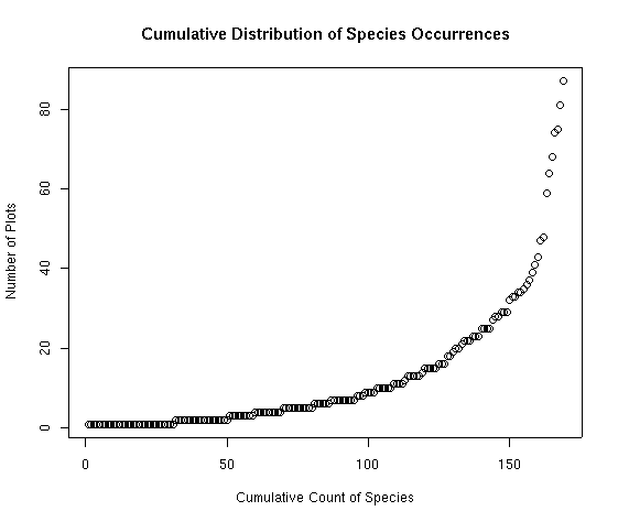
The figure above portrays a fairly typical distribution of species abundances. Note that the distribution is seriously skewed. We can correct for that by putting the Y axis on a log scale to achieve a semi-log plot.
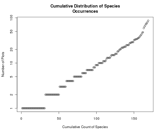
Notice how the Y axis is now log-scaled but retains the units in the original scale. If we had just plotted the log species abundances we would get
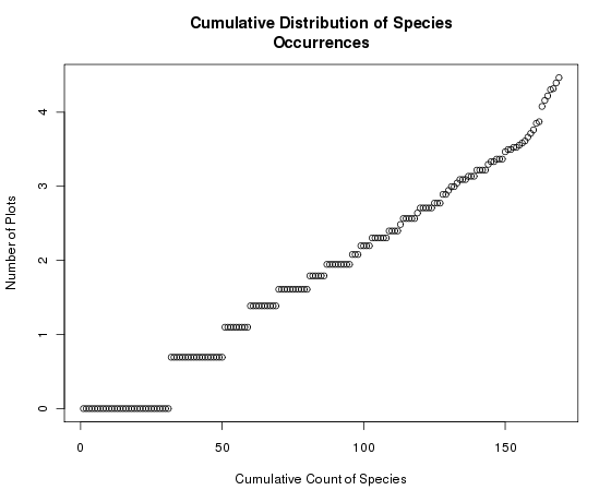
Notice here that the graph itself has not changed, but the Y axis is now scaled 0-4 (log of spc.pres), instead of 1-100. Generally, we want to transform the axis and keep the units in the original scale.
Many people are more familiar with looking at such distributions as histograms, so a short explanation is probably in order. Along the X axis is the number of species at or below a specific Y value. For example, approximately 100 out of 169 species occur in 10 or fewer plots; 130 of the species occur in 20 or fewer plots. To see the exact distributions, use the seq() function as follows:
which shows that first 102 species occur less than 10 times, species 103-108 occur exactly 10 times, and species 109-169 occur more often than 10 times. Let's look at this expression a little closer. The second half (the logical subscript) we have seen before, i.e. [sort(spc.pres)==10] means "those species which occur 10 times". For example, to see their names,
agrdas asthum astmeg erifla eriumb tradub
    10     10     10     10     10     10
Generally stated, most species occur infrequently, and a few are quite common. Only two species (Carex rossii and Symphoricarpos oreophilus) occur in half or more of the sample plots. To see the actual distribution, with species names attached, simply enter
 chrdep shearg arcuva atrcon agrscr phlpra anemul artcar astchi astten dessop
      1      1      1      1      1      1      1      1      1      1      1

 echtri erieat erisub genaff gerric heddru ivesab leueri ligpor litinc lygspi
      1      1      1      1      1      1      1      1      1      1      1
             .                         .                            .
             .                         .                            .
             .                         .                            .
 tetcan erirac artarb juncom chrvis oryhym sithys pacmyr ceamar purtri berrep
     35     36     37     39     41     43     47     48     59     64     68

 arcpat senmul symore carrss
     74     75     81     87
For comparison, the following figure is the same data in histogram form, plotted with
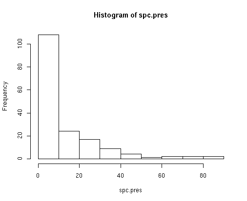
Whittaker (19xx) suggested that species abundance distributions sometimes follow a log-normal distribution. We can easily convert the plot to log distributions as shown below.
The figure below shows the histogram of the natural log of the spc.pres distribution.
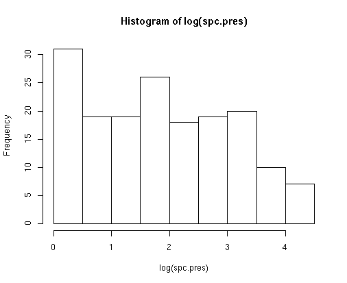
Clearly, even after log transformation, the number of species with very few occurrences is higher than we would expect for any sort of normal distribution.
What is the mean cover of each species when it occurs (not averaging zeros for plots where it is absent)?
Here we simply use the apply() function to calculate the sums of the columns of the matrix veg, and then divide by the number of plots in which that species occurs.spc.abund <- apply(cover,2,sum) spc.mean <- spc.abund/spc.pres # to get the average cover for each species
spc.abund <- colSums(cover)
spc.mean <- spc.abund/spc.pres      # to get the average cover for each species
to see the ECDF of species mean abundances
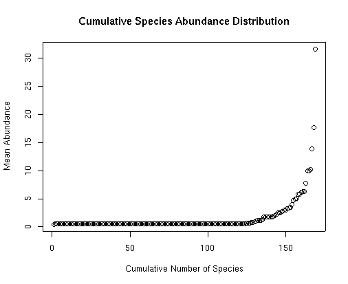 Notice that this distribution is even more extreme than the previous ECDF for
occurrence. Most species only occur at very low abundance, while relatively
few are abundant (only four species with average cover > 10%). Perhaps more
interesting than the simple distribution of mean abundance is the following.
Notice that this distribution is even more extreme than the previous ECDF for
occurrence. Most species only occur at very low abundance, while relatively
few are abundant (only four species with average cover > 10%). Perhaps more
interesting than the simple distribution of mean abundance is the following.
Is the mean abundance of species correlated with the number of plots they occur in?
To examine this question we can plot the species mean abundance (spc.mean) as a function of the species occurrences (spc.pres) as follows.
then click next to a point and its number will appear. If you use a third argument, you can get the name of the species printed next to the dot. For example
will print the name of the species next to its dot, as names(veg) is the R function to get the columns names of the the veg matrix.
Click the second mouse button (or hit 'ESC' on some operating systems)
to stop listing points. The numbers of the selected points are
listed in the order selected at the command line, and can be stored in a vector as follows:
The distribution shown is actually quite interesting. Most of the widespread
species (Carex rossii, Symphoricarpos oreophilus, Senecio multifida and
Berberis repens) have low mean abundance. Only Arctostaphylos
patula is both widespread and abundant. In contrast, some other species
(e.g. Artemisia arbuscula/nova, Stipa comata, and Quercus
gambelii) are much less widespread, but abundant (if not dominant) when
present. Arguably, species which are widespread or abundant (if not both),
give an area's vegetation much of its character, while those species which are
locally distributed may highlight sites of specific interest and add the
interesting detail to the study of vegetation. We'll cover a little more of
this discussion with some new functions below.
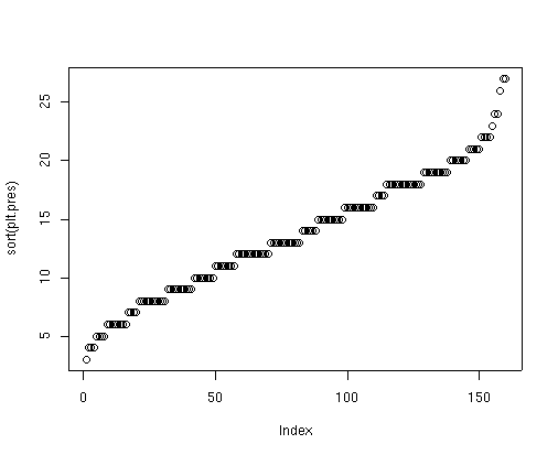
Surprisingly, perhaps, the number of species per plot ranges from 3 to 27
species per 0.1 acre. Bryce Canyon includes some rapidly eroding, xeric
badlands where very few species can survive, leading to the plots with
relatively few species. Alternatively, the most species rich sites are
generally xeric shrubfields dominated by Artemisia arbuscula/nova or
harsh woodland sites dominated by Picea pungens and Juniperus
communis. Many Rocky Mountain ecologists would be surprised to see
Picea pungens described as a harsh woodland species, but that describes
much of its distribution in Bryce Canyon.
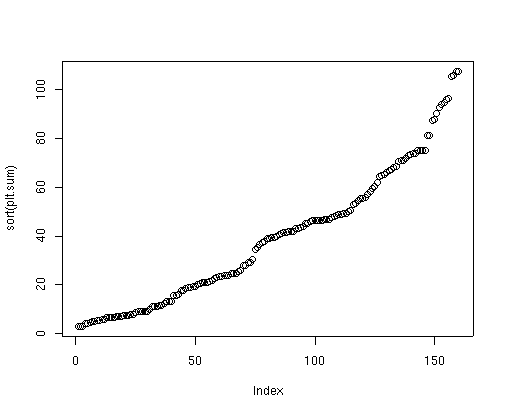
To plot the total cover on each plot, first calculate the vector of plot cover as follows:
Again, perhaps surprisingly, total cover per plot ranges from a minimum of 3%
to just greater than 100% (107.5). As the species are estimated individually
and then summed, it is easily possible to get more than 100% cover in a single
plot, but few plots in Bryce Canyon achieve this high a total cover. In
addition, using the cover class midpoint as the estimated cover in the sums is
very likely biased too high (the discussion is too detailed to get into here),
and yet the values are still quite low. Bryce Canyon is dominated by xeric
sites with relatively low total plant species abundance.
Finally, to answer our question on the relation between total cover and number of species/plot,
Apparently, there is very little relationship between the number of species per plot and the total cover.
This is not completely surprising since we already established that one of the most species-rich communities
was a harsh site woodland. Still it is somewhat surprising that the sites with highest cover have fewer than
the average number of species per plot.
Storing our calculated vectors in a list will make them more easily accessible
in the future, but is not really required, as R always saves all calculated
data in the workspace, and asks whether to save your workspace when you exit R.
Any time you identify a series of plots or analyses that you are likely to
repeat, or that others are likely to use, you should think about writing a
function to automate the process, and then distribute that function, possibly
as an R package. Accordingly, I have developed an a function to repeat a
variation on the analyses we just performed, called abuocc() which is
in the labdsv package. To repeat the analysis, (since we have already loaded
labdsv), simply enter
and hit return as prompted. Two things you should note: (1) we could have
simply done this from the beginning, but then you wouldn't have learned nearly
as much R, and (2) the plots are organized slightly differently. For example,
in several of the plots the Y axis is now log-scaled. In addition, many of the
plots now go from maximum to minimum. This is in accordance with many studies
of "niche theory," and is probably more easily visualized. To understand the
differences in R, simply study the function code appended below.
In Lab 2 we will explore the site data from Bryce Canyon.
Is the total abundance of vegetation correlated with the number of species in a plot?
To calculate this, we will again use the apply function, this time applied to the rows rather than columns
of data frame veg.
plt.pres <- apply(cover>0,1,sum) # to calculate the number of species in each plot
                                 # or
plt.pres <- rowSums(cover>0)
plot(sort(plt.pres))             # to see the ECDF of number of species/plot
plot(plt.pres,plt.sum,xlab='Sample Plot Species Richness',
                      ylab='Sample Plot Total Cover')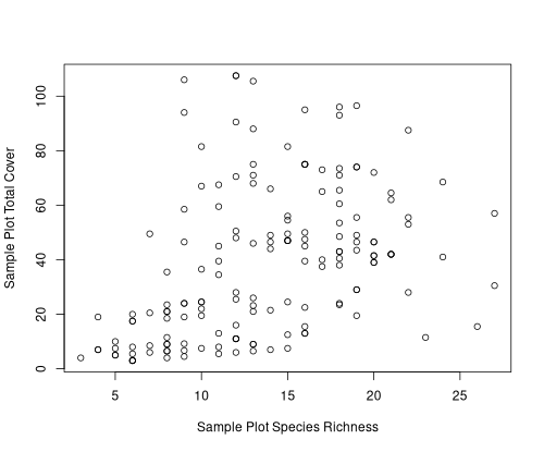
plt.pres[plt.sum>100]
                             # or
subset(plt.pres,pltsum>100)
bcnp_18 bcnp_19 bcnp_20 bcnp_90
     12      13       9      12
spc.dat<-list(spc.pres=spc.pres,spc.mean=spc.mean,plt.pres=plt.pres,
              plt.sum=plt.sum)
Species Abundance Calculations
I believe that the analyses we just performed (which I will call
abundance/occurrence analysis) are highly informative and should be computed
and plotted for any community dataset before beginning detailed analyses of
the community. In later labs, I will demonstrate that the characteristics
apparent in this plot are highly influential on the statistical power and
suitability of many analyses.
Next Lab
Functions included in this lab
abuocc <- function (comm, minabu = 0, panel = "all")
{
    if (!is.data.frame(comm))
        comm <- data.frame(comm)
    spc.plt <- apply(comm > minabu, 1, sum)
    plt.spc <- apply(comm > minabu, 2, sum)
    if (minabu == 0) {
        mean.abu <- apply(comm, 2, sum)/plt.spc
    }
    else {
        mean.abu <- rep(0, ncol(comm))
        for (i in 1:ncol(comm)) {
            mask <- comm[, i] > minabu
            mean.abu[i] <- sum(comm[mask, i])/max(1, plt.spc[i])
        }
    }
    mean.abu[is.na(mean.abu)] <- 0
    if (panel == "all" || panel == 1) {
        plot(rev(sort(plt.spc[plt.spc > minabu])), log = "y",
            xlab = "Species Rank", ylab = "Number of Plots",
            main = "Species Occurrence")
        if (panel == "all")
            readline("Press return for next plot ")
    }
    if (panel == "all" || panel == 2) {
        plot(rev(sort(spc.plt)), xlab = "Plot Rank", ylab = "Number of Species",
            main = "Species/Plot")
        if (panel == "all")
            readline("Press return for next plot ")
    }
    if (panel == "all" || panel == 3) {
        plot(plt.spc[mean.abu > minabu], mean.abu[mean.abu >
            minabu], log = "y", xlab = "Number of Plots", ylab = "Mean Abundance",
            main = "Abundance vs Occurrence")
        yorn <- readline("Do you want to identify individual species? Y/N : ")
        if (yorn == "Y" || yorn == "y")
            identify(plt.spc[mean.abu > minabu], mean.abu[mean.abu >
                minabu], names(comm)[mean.abu > minabu])
        if (panel == "all")
            readline("Press return for next plot ")
    }
    if (panel == "all" || panel == 4) {
        plot(spc.plt, apply(comm, 1, sum), xlab = "Number of Species/Plot",
            ylab = "Total Abundance")
        yorn <- readline("Do you want to identify individual plots? Y/N : ")
        if (yorn == "Y" || yorn == "y")
            identify(spc.plt, apply(comm, 1, sum), labels = row.names(comm))
    }
    out <- list(spc.plt = spc.plt, plt.spc = plt.spc, mean = mean.abu)
    attr(out, "call") <- match.call()
    attr(out, "comm") <- deparse(substitute(comm))
    attr(out, "timestamp") <- date()
    attr(out, "class") <- "abuocc"
    invisible(out)
}
matrify <- function (mat)
{
    if (ncol(data) != 3)
        stop("data frame must have three column format")
    plt <- mat[,1]
    spc <- mat[,2]
    abu <- mat[,3]
    plt.codes <- levels(factor(plt))
    spc.codes <- levels(factor(spc))
    taxa <- matrix(0,nrow=length(plt.codes),ncol=length(spc.codes))
    row <- match(plt,plt.codes)
    col <- match(spc,spc.codes)
    for (i in 1:length(abu)) {
        taxa[row[i],col[i]] <- abu[i]
    }
    taxa <- data.frame(taxa)
    names(taxa) <- spc.codes
    row.names(taxa) <- plt.codes
    taxa
}
reconcile <- function (comm, site, exlist = 10)
{
    if (identical(row.names(comm), row.names(site))) {
        cat("You're good to go\n")
    }
    else {
        orig_comm <- deparse(substitute(comm))
        orig_site <- deparse(substitute(site))
        extracomm <- nrow(comm) - sum(row.names(comm) %in% row.names(site))
        if (extracomm > 0) {
            cat(paste("You have", extracomm, "plots in comm not in site\n"))
            if (extracomm <= exlist)
                print(row.names(comm)[!row.names(comm) %in% row.names(site)])
            cat("I'll delete the extra plots in comm in the output\n")
        }
        extrasite <- nrow(site) - sum(row.names(site) %in% row.names(comm))
        if (extrasite > 0) {
            cat(paste("You have", extrasite, "plots in site not in comm\n"))
            if (extrasite <= exlist)
                print(row.names(site)[!row.names(site) %in% row.names(comm)])
            cat("I'll delete the extra plots in site in the output\n")
        }
        if (!extracomm && !extrasite) {
            cat("Your data.frames have the same sample units\n")
            cat("but are sorted differently\n")
            cat("I'll fix that\n")
        }
        if (!extracomm || !extrasite) {
            cat("Your edited data.frames now have the same sample units\n")
            cat(" but are sorted differently\n")
            cat("I'll fix that\n")
        }
        comm <- comm[order(row.names(comm)), ]
        site <- site[order(row.names(site)), ]
        comm <- comm[row.names(comm) %in% row.names(site), ]
        site <- site[row.names(site) %in% row.names(comm), ]
        out <- list(comm = comm, site = site)
        attr(out, "call") <- match.call()
        attr(out, "orig_comm") <- orig_comm
        attr(out, "orig_site") <- orig_site
        invisible(out)
    }
}